SVS (SmartVision Studio)

Product Overview

The vision algorithm development platform SmartVision Studio (hereinafter referred to as "SVS") is a vision algorithm development platform independently developed by APLUX, consisting of image processing operators and interactive visual function modules. The platform is feature-rich and easy to use, helping developers quickly build various vision solutions such as localization, measurement, defect detection, and information recognition by dragging and connecting nodes.

How It Works

Plain

Acquire Image → Preprocessing → Localization/Matching → Measurement/Detection → Result Filtering/Judgment → Output (Image/IO)

A workflow uses nodes as its basic units: each node represents a function module, nodes are related by input and output connections, and the whole flow is edited on the canvas and executed with a single click.

Quick Start

This document walks you through your first detection flow from scratch: Image Source → DL Localization → Contour Detection → Contour Cropping → Result Rendering. The whole process takes about 5 minutes.

Step 1: Start the Software

Confirm that the SVS service is running on the device (default backend port 58300).
Open the front-end page in a browser (the development environment defaults to http://{ip}:58300; in production, use the deployed address).
Once the page is loaded, you enter the main workflow editing interface; no login is required.

Step 2: Create a New Workflow

Click New Workflow in the top action bar.
Enter a workflow name in the dialog that appears (for example, "Quick Start") and click OK.
A blank flow page named Main Flow appears on the canvas.

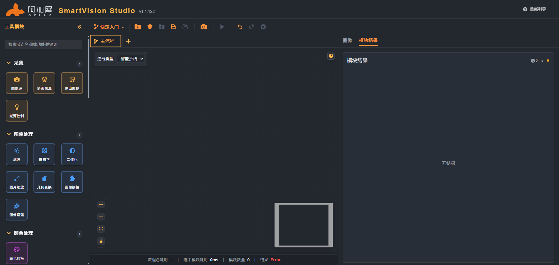
Step 3: Add an Acquisition Node

In the Tool Module panel on the left, find Image Source under the Acquisition category.
Press and hold Image Source, drag it to an empty area of the canvas, and release; the node appears on the canvas.

The node requires a configured camera or static image before it can run; see Image Source for details.

Configure the image source parameters and select a camera (C0 Camera, C1 Camera, C2 Camera); the C0 Camera is used by default.

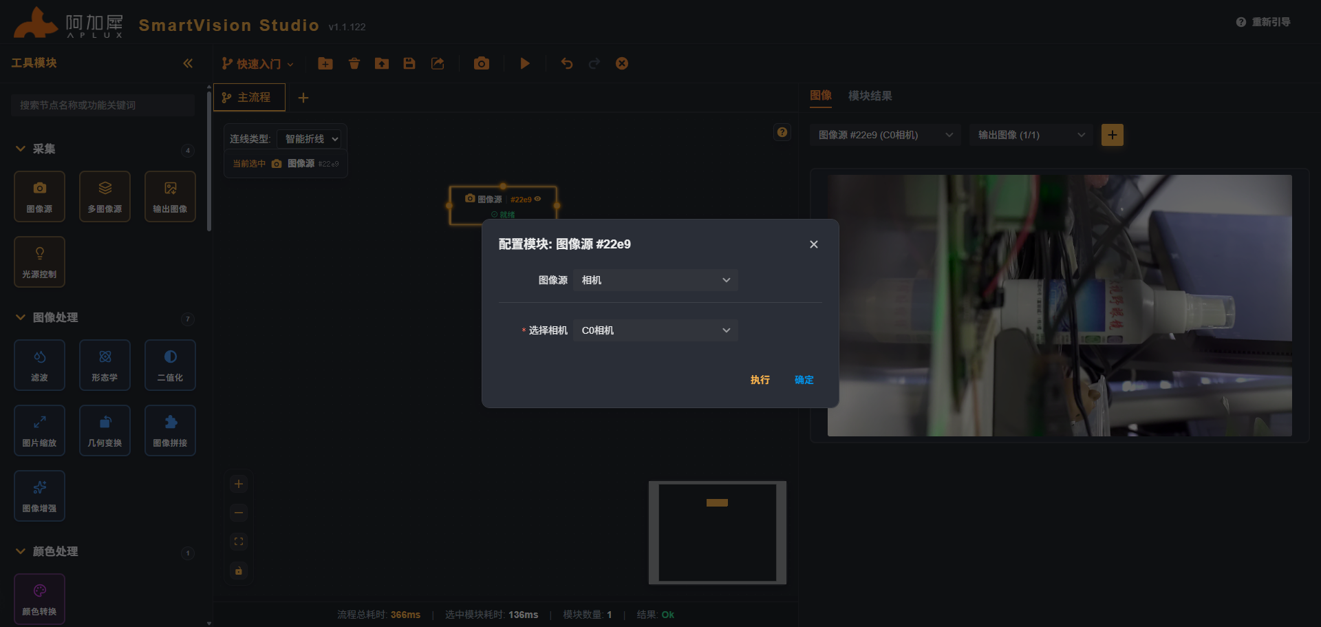
Step 4: Add Tool Modules

Drag Localization, Contour Detection, Contour Cropping, and Result Rendering onto the canvas and connect them.

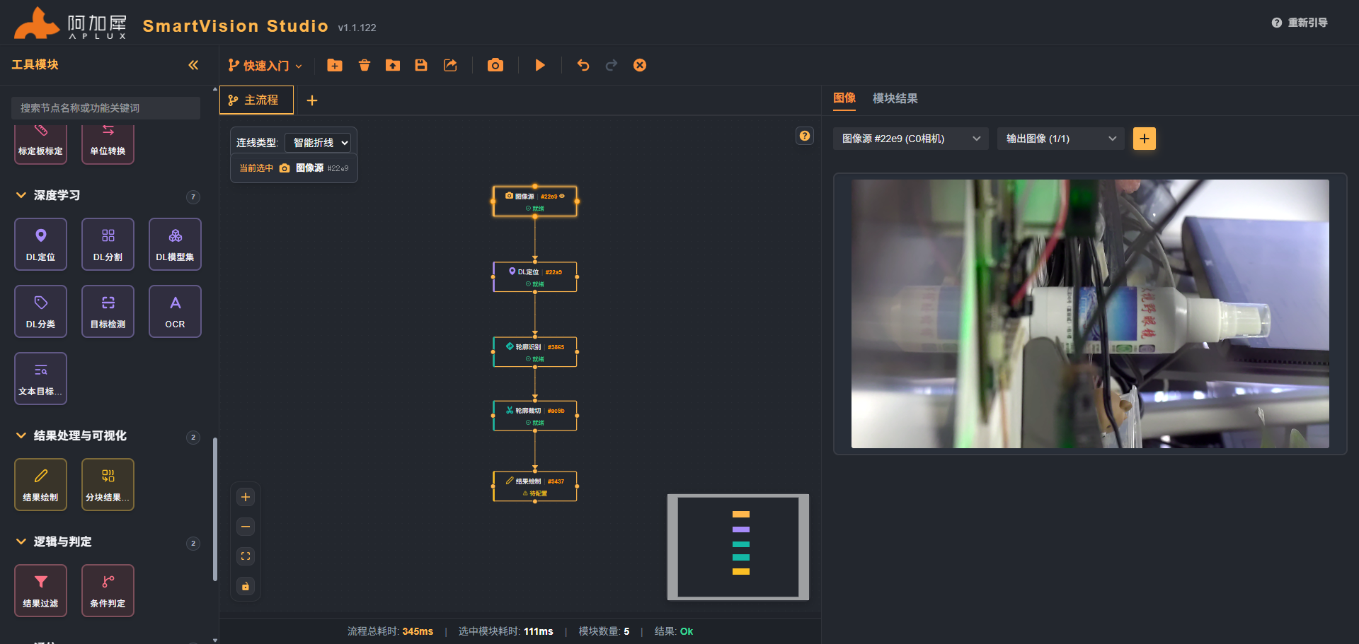
Download the model trained with AIC to the local device (see the Deep Learning section for details) and upload the localization model.

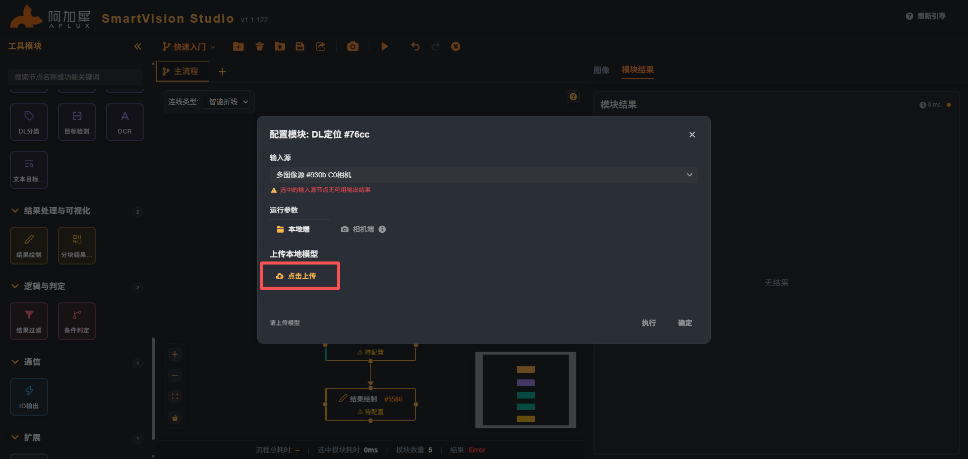
Step 5: Execute the Workflow

Click the Execute button in the top action bar.
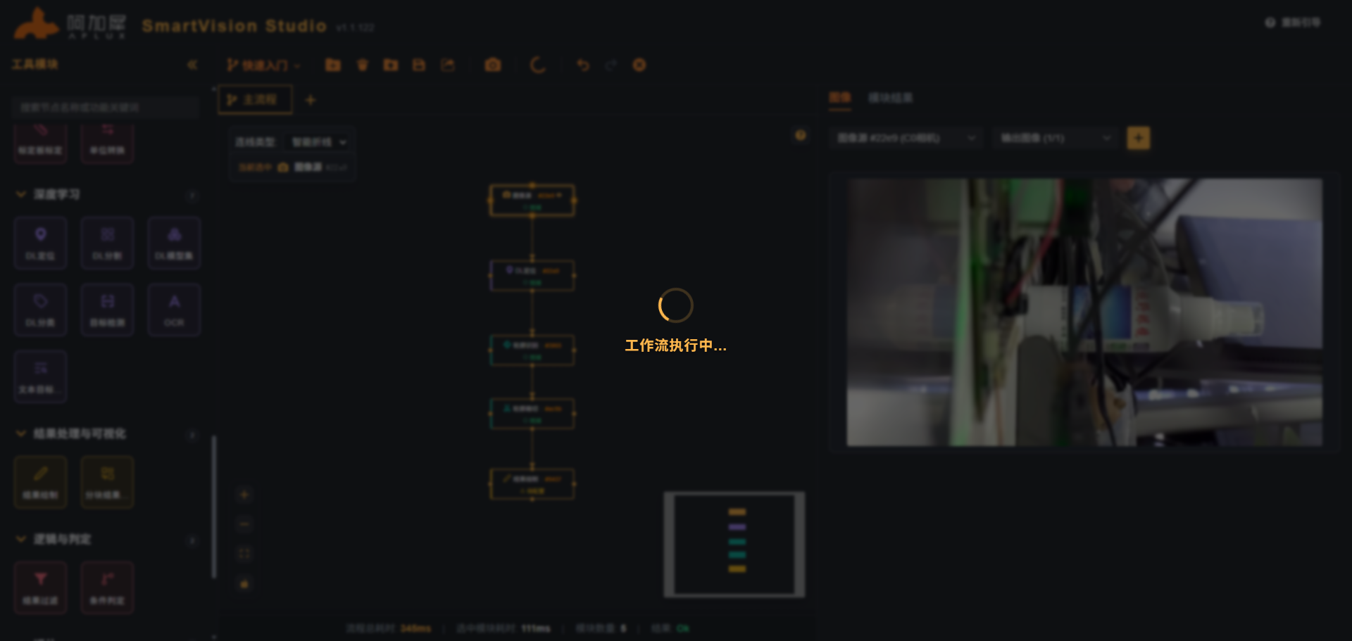
During execution, the page shows an overlay with the message "Workflow executing...".

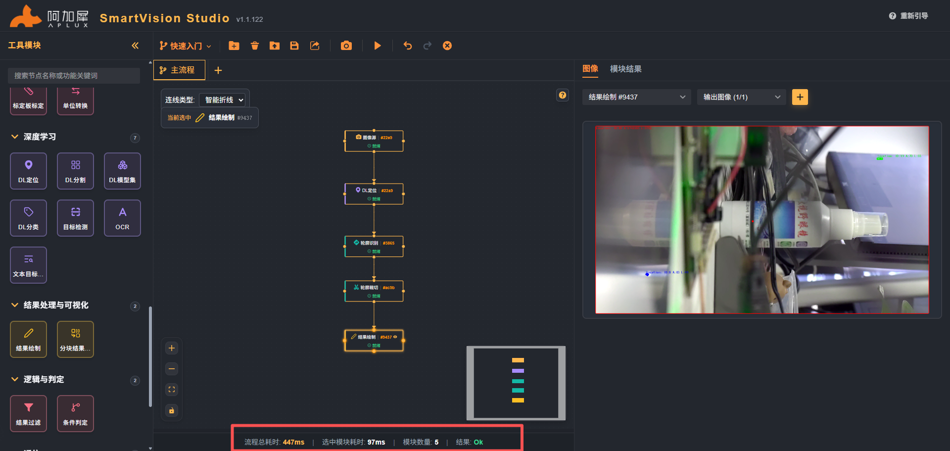
After execution finishes, the bottom summary bar shows the total flow duration, the module count, and the result status.

Step 6: View the Results

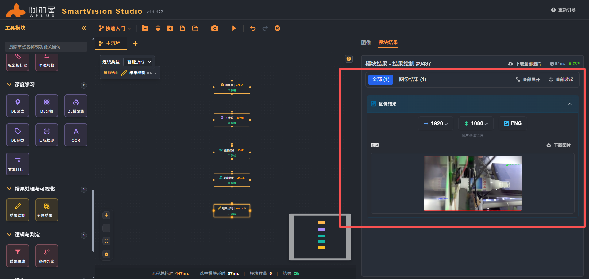
Switch the right panel to the Image tab to view the output image.

Step 7: Export App

Export the successfully running flow as an app to SVE (see the Scheme Global Functions - Export App section for detailed steps).

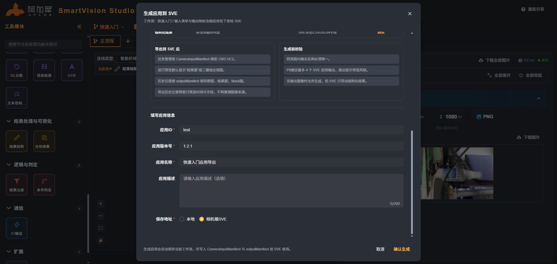
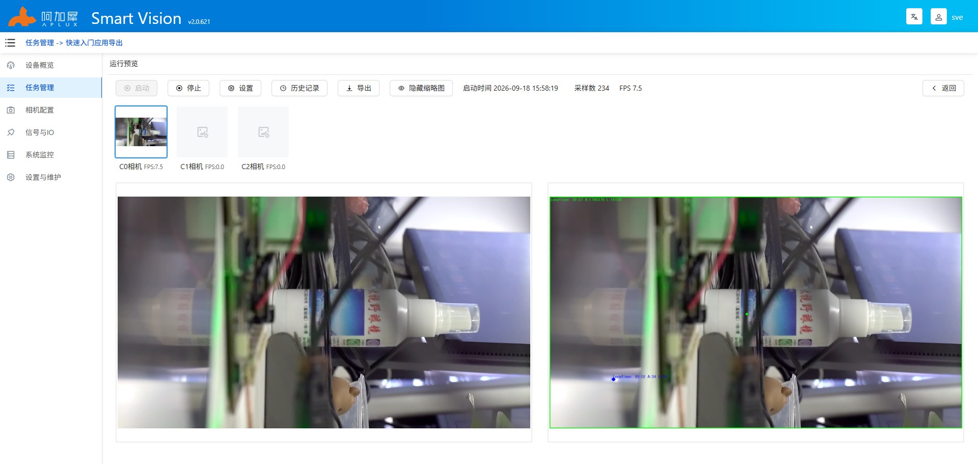
Visit the camera IP at port 58200 in a browser, click to start the pushed app, and then run the preview.

Next Steps

Learn about each interface area: Interface Introduction
More workflow operations: Scheme Composition Introduction
Parameter tuning and troubleshooting (single-node execution, result verification, duration analysis): Debugging and Running
Browse all modules: Module Introduction

Interface Introduction

This chapter introduces the overall interface layout of the SmartVision Studio (SVS) platform and the functions of each area, helping users get familiar with the interface structure and quickly start building and debugging workflows.

Interface Layout

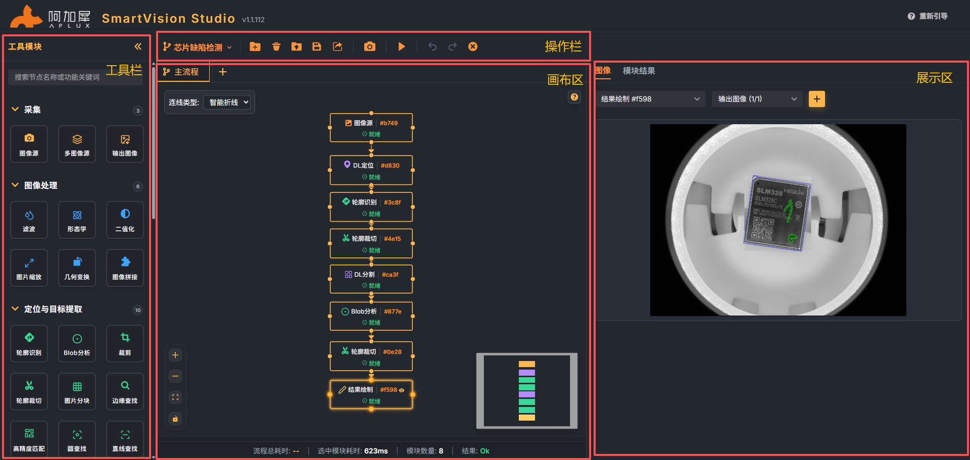
SmartVision Studio uses a four-area layout:

Toolbar: A draggable node module library; modules can be dragged or double-clicked into the workspace
Action Bar: Workflow-level quick action buttons
Canvas Area: The main workspace for flow design and node editing, supporting multi-flow tab switching
Display Area: For viewing image output and module execution results

Action Bar

It consists of two parts, as shown below:

Workflow Name Area: Displays the current workflow name and supports the following operations.

Function	Operation	Detailed Description
Rename Workflow	Double-click the workflow name	1. A "Rename Workflow" dialog appears 2. Enter a new name 3. Click "OK" 4. The system checks whether a workflow with the same name exists on the camera 5. If the name is duplicated, a warning is displayed and saving is blocked
View Flow List	Hover the mouse over the workflow name	- A flow list popup appears - Shows all flow names (currently only 1 main flow is supported) - Click a flow name to reopen that flow tab

Common Function Buttons Area: Provides quick access to some frequently used functions.

Each function button can be operated by single-clicking it; brief descriptions are as follows:

Icon	Name	Operation Description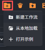
	New Workflow	1. A "New Workflow" dialog appears 2. Enter a workflow name 3. Click "OK" to complete the creation 4. The main flow is created automatically and enters editing
	Load Workflow from Local	1. Triggers the file selection dialog 2. Select a workflow file in `.json` format 3. The system automatically parses and loads the workflow onto the canvas
	Open Example	Open the built-in example app
	Export Workflow to Local	Export the current workflow as a local `.json` file
	Save to Camera	Save the current workflow to the camera
	Generate Application	When the canvas is not empty and contains only one complete flow chain, exports the workflow as a standalone app This operation automatically saves the workflow to the camera
	Global Camera Settings	See the "Global Camera" section for details
	Execute Current Workflow	The canvas is not empty and contains only one complete flow chain. 1. The button turns into a spinning animation 2. A full-screen semi-transparent overlay with the "Workflow executing..." message is displayed 3. The overlay closes automatically after execution 4. The results are shown in the right result panel This operation automatically saves the workflow to the camera
	Undo	When there are undoable historical operations, undoes the last canvas operation
	Redo	When there are undone operations, redoes the undone operations
	Clear Canvas	Clear all nodes and connections in the current flow
	Delete from Camera	1. A "Delete from Camera" dialog appears 2. The list shows all workflows on the camera 3. Click to select the workflow to delete 4. Click the "Delete" button 5. Confirm to delete

Tool modules are divided into thirteen major categories by function; see the Module Introduction section for details:

Category	Module Count	Description
Acquisition	4	Acquisition modules are used to obtain image input sources, supporting real-time camera acquisition, switching between multiple image sources, and static image import. Each workflow must contain one acquisition node as its starting point.
Image Processing	7	Image processing modules provide basic image preprocessing and transformation functions, including filtering and denoising, morphological operations, binarization, scaling, geometric transformations, and image composition.
Color Processing	1	Color processing modules are used for color space conversion, supporting conversion of RGB color images into grayscale, HSV, HSI, or YUV images.
Localization and Target Extraction	10	Localization and target extraction modules are the core of visual inspection, including various localization algorithms such as circle finding, line finding, edge finding, contour detection, and Blob analysis.
Matching	4	High-Precision Matching, Contour Matching, Fast Matching, Grayscale Matching
Measurement	6	Measurement modules are used to calculate geometric distances between feature points/lines in an image, supporting point-point measurement, point-line measurement, line-line measurement, line-circle measurement, circle-circle measurement, and point-circle measurement.
Calibration and Coordinates	2	Calibration Board Calibration, Unit Conversion
Recognition and Code Reading	1	Recognition and code reading modules are used to recognize and read the encoded content of code symbols from the input image.
Deep Learning	7	Deep learning modules integrate AI inference capabilities, supporting various models such as object detection, classification, segmentation, and OCR, as well as text object detection.
Result Processing and Visualization	2	Result processing modules are used to render detection or measurement results onto the output image for visual verification.
Logical Judgment	2	Logical judgment modules are used for conditional filtering and logical judgment of detection results, supporting two modes: result filtering and condition judgment.
Communication	1	Communication modules are used for IO signal interaction with external devices.
Extension	1	Extension modules support custom processing logic and can load user-defined models or algorithm libraries.

Canvas Area

The canvas area is the core area for building, editing, and managing workflows. Users can complete the construction of a vision algorithm processing flow by dragging module nodes, creating connections, and configuring node parameters.

Flow Tab Operations

Function	Operation	Detailed Description
New Flow	Click the `+` button at the far right of the tab bar	1. A "New Flow" dialog appears 2. Enter a flow name 3. Click "OK" to create 4. The new flow tab opens automatically The current version only supports using the default main flow; creating additional flows is not allowed for now. The multi-flow feature will be available in a later version.
Switch Flow	Click a flow tab	- The canvas switches to the corresponding flow - The image source and result panel on the right refresh automatically - Each flow independently remembers its image source selection state
Rename Flow	Double-click the flow tab name	1. A "Rename Flow" dialog appears 2. Enter a new name 3. Click "OK" to complete the renaming
Delete Flow	Click the delete icon (trash can) on the tab	1. A confirmation box appears: "Delete this flow?" 2. Click "OK" to permanently delete the flow

Module Node Operations

Function	Operation	Detailed Description
Add Module Node	Select a tool module and drag it to the canvas area	1. Press the left mouse button on the node module 2. Keep it pressed and move the mouse to the canvas 3. Release the mouse at the target position 4. The node is automatically generated at the release position Each flow can have only one acquisition node (camera or static image); adding another one prompts an error.
Single-Click Module Node	Left-click the node	- The node border is highlighted - The right display area automatically refreshes with the node's output results - The node's output result data is requested automatically This operation automatically saves the workflow to the camera
Double-Click Module Node	Left double-click the node	A node configuration dialog appears; click the "Execute" or "OK" button. This operation automatically saves the workflow to the camera
Drag Module Node	Press and hold the node and drag it	- The node position moves in real time - Connected edges follow and adjust automatically
Right-Click Selection	Right-click the node	The node is selected and highlighted with a dashed border
Right-Click Multi-Selection of Nodes	Right-click multiple nodes one by one	All right-clicked nodes are selected
Long-Press Right-Button Drag	Press and hold the mouse right button and drag to box-select nodes	All box-selected nodes and connections are selected
Delete Node	After right-click selecting a node, a delete action panel appears automatically	Delete all selected nodes
Deselect	Click an empty area of the canvas	Deselect all nodes and hide the delete panel automatically
Create Connection		1. Hover over a node to show its connection points 2. Press a connection point and drag 3. Move to the target node's connection point 4. Release the mouse to complete the connection
Delete Connection	Right-click a connection and select "Delete"	Delete the connection

Bottom: Summary Bar

Shows the running statistics of the current flow:

Total flow duration
Duration of the selected module
Module count
Result status (Success/Failure)

Display Area

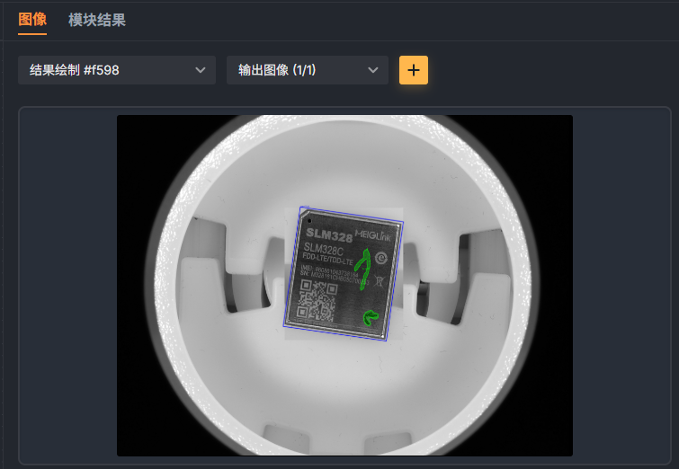
It contains two parts:

Image: Shows the output image of the currently selected module. After the whole workflow has been executed, the output images of all modules involved in the flow can be selected and displayed in the drop-down box. Options follow this format: Module Node Name #Short ID.Output Image (1/N); for example, DL Model Set #fbec .Output Image (1/2) means that the DL Model Set module has the ID #fbec, its module has 2 output images in total, and currently its 1st image is displayed.
Module Results: Shows the output result data of the currently selected module; different modules display different result data. See the "Module Introduction" section for details.
- Supports filtering results by type
- Supports expand all/collapse all
- Supports downloading images or exporting data

Image Output

When the "Image" tab is selected, the system shows the image information of the current module and its upstream modules (if the upstream modules have image output). Users can select the images to view via checkboxes, and the system displays the selected image content accordingly.

As shown below:

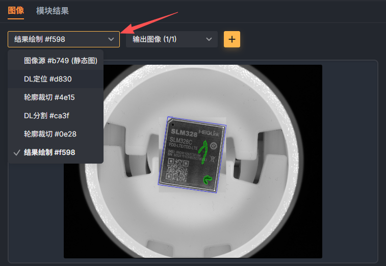
When the image source is a "static image", the display area provides static image list management; see the "Image Source" module section for details.

Module Results

After a module finishes running, the system shows the module's running results in the module output panel on the right. The module results area mainly consists of two parts:

Top Area: Shows the module's running information (such as status and duration).
Main Content: Shows the computation output results corresponding to the module.

As shown below:

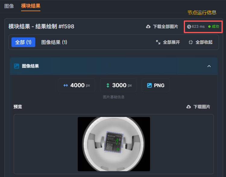
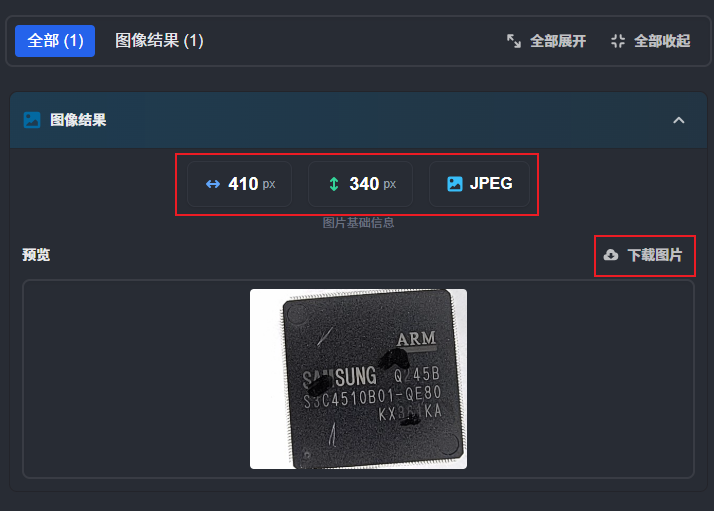
For most image-centric modules (for example: Image Source, Crop, Image Filtering, Morphological Processing, Binarization, etc.), the output results are mainly images. The interface shows the following information about the image:

Image Size: Shows the width and height of the image.
Image Format: Shows the encoding format of the current image (such as JPG, PNG, BMP, etc.).
Image Operations:
- Download Image: Save the output image locally.
- Zoom Preview: Supports full-screen or partial zoom-in viewing for observing details.

As shown below:

Apart from image results, other modules also output additional information; see the Module Introduction section for details.

Scheme Composition Introduction

Flow Management

A workflow is used to organize and execute visual processing and inference flows. According to inspection requirements, users can build an algorithm scheme by dragging modules, creating connections, and setting parameters.

Workspace Area

After creating a new workflow, select the required tool modules from the left toolbar and drag them into the main flow workspace area to form a complete workflow.

The main flow area supports various editing and view operations, including: connection type switching, zoom in/out, fit to view, lock modules, making it convenient for users to flexibly adjust the flow structure and layout.

As shown below:

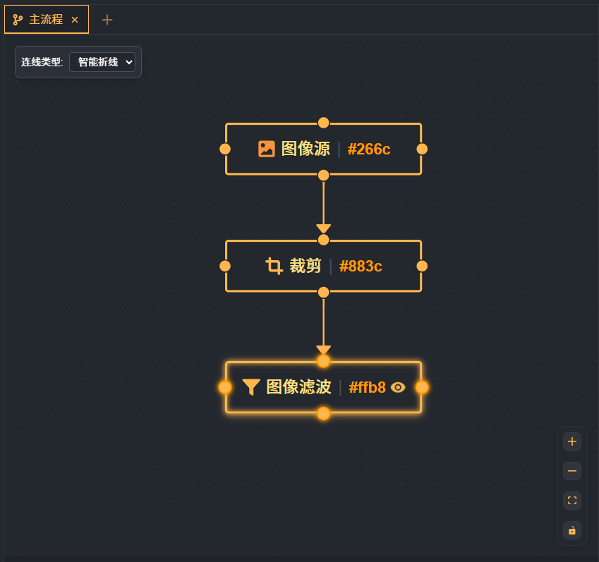
Connection type: Modifies the connection style between modules. Supports three types: smart polyline, straight line, curve, making it easy to choose the appropriate display method based on flow complexity.
Zoom in: Enlarges the current workspace area, making it easy to view details or perform precise module operations.
Zoom out: Shrinks the workspace area, suitable for viewing the overall flow structure.
Fit to view: Automatically adjusts the view scale and module sizes to quickly locate the optimal display range of the current workflow.
Lock modules: Once locked, modules cannot be dragged or repositioned, preventing accidental operations.

Flow Error Notification

During workflow construction, if some modules are incompletely configured, models are missing, or dependent upstream nodes are abnormal,

the system highlights the error state in the main flow area to help users quickly locate the problem.

As shown below:

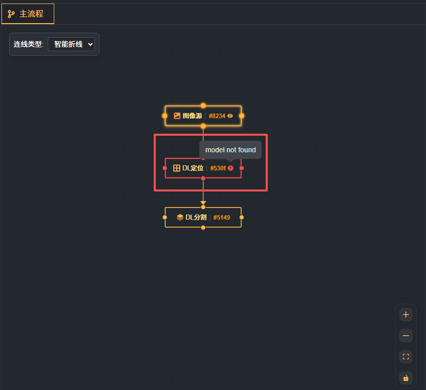
When a module has an error, the system marks the node with a red border and red icon, and displays detailed error information on mouse hover.

Module General Configuration

Basic Parameters

Image Source: By default, subscribes to the output image of the preceding module.

Runtime Parameters

Runtime Parameters: Sets the algorithm parameters for the module during visual inspection, so as to achieve the desired detection effect. Runtime parameters differ by module; refer to the actual module content for details.

Scheme Global Functions

Export App

The Export App function is used to package the current workflow into an independent deployable app.

This makes it convenient to run directly on other devices without re-editing the workflow. As shown below

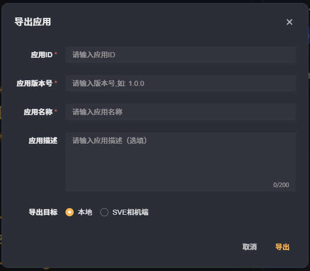
In the Export App interface, you need to fill in the basic app information and export target:

App ID: Required. The unique identifier of the app, used to distinguish different apps. English letters or numeric combinations are recommended.

App Version: Required. The app version number; the recommended format is major.minor.patch (for example: 1.0.0). Used for version management and update records.

App Name: Required. The display name of the app, used to identify the app after export.

App Description: A brief description of the app's function, purpose, or algorithm flow (max 200 characters), for convenient later maintenance and identification.

At the bottom of the interface, you can select the Export Target to specify where the app is exported:

Local: Export the app to the local computer, generating an independent app package file (usually in .zip format). Suitable for offline deployment, backup, or transfer to other devices.
SVE Camera: Push the app directly to the local SVE camera device. The system performs the transfer and deployment automatically; once complete, the app can be run directly on the camera.

Global Camera

Global Camera management is used to uniformly configure, manage, and debug all connected camera devices. Configuring camera parameters in this interface ensures stable and consistent image acquisition, thereby improving the accuracy and reliability of subsequent algorithm processing results.

Users can view, select, and adjust the basic parameters and color parameters of each camera in this module to meet different algorithm task requirements.

As shown below:

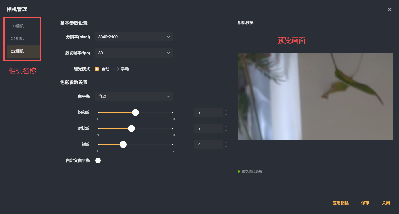
Camera List

The left side of the interface displays a list of all recognized camera devices, for example: C0 Camera, C1 Camera, C2 Camera.

Tip: Camera numbers and cable/device interfaces should be marked correspondingly during on-site installation, to avoid confusion in later debugging.

Click any camera name to enter the corresponding parameter settings interface and preview image.

Basic Parameter Settings

The right area is the detailed parameter configuration area of the current camera, divided into two parts: Basic Parameter Settings and Color Parameter Settings.

Resolution(pixel): Sets the resolution of the camera output image. Supports multiple standard resolution options (such as 3840×2160, 1920×1080, etc.).

Trigger Frame Rate (fps): Sets the frame rate of the camera, that is, the number of frames captured per second. A higher frame rate gives a smoother image, but may increase system load. Such as 60fps, 120fps

Exposure Mode: Supports two modes: "Auto" and "Manual".

Auto Mode: The system automatically adjusts exposure according to lighting conditions.
Manual Mode: Users can set the exposure duration, exposure level, and exposure compensation themselves to achieve precise control.

Color Parameter Settings

Auto White Balance

Sets the white balance mode of the camera. Supports:

Auto: The system automatically adjusts color temperature balance;
Manual: Users can customize white balance parameters.

Image Adjustment Parameters

Parameter Name	Range	Description
Saturation	0 – 100	Controls the vividness of image colors.
Contrast	0 – 100	Controls the contrast strength of light and dark levels in the image.
Sharpness	0 – 100	Controls the clarity of image edges

Custom White Balance

When Auto White Balance is turned off, white balance parameters can be set manually, which is suitable for scenarios with fixed light source conditions. Supports setting RGB gain and color temperature adjustment.

Common Node Parameters: ROI

Most positioning and detection nodes support ROI settings, which are used to limit the detection range:

Expand ROI settings in the configuration dialog to switch between "Manual" and "Full Frame".
Manual mode supports shapes such as rectangle, polygon, line caliper, circle caliper, and arc caliper (the shapes supported differ by module).
ROI parameters such as start point, width/height, radius, and caliper count change dynamically with the shape.

Module Introduction

Acquisition

Modules under the Acquisition category configure image input sources.

Image Source

The Image Source module provides image sources, with options for Local Image or Camera.

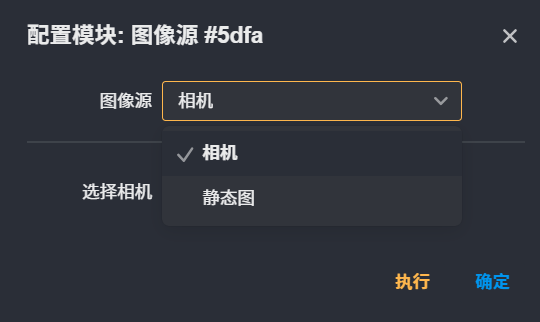
Parameter Configuration
- When the image source is set to Camera, images are obtained from configured cameras. The following parameters need to be set:
  - Select Camera: Select the associated camera. Click the "Execute" button to capture one frame from the corresponding camera and display it in the image area. For camera configuration, see the "Global Camera" section.
- When the image source is set to Local Image, images are loaded from local storage. The following parameters need to be set:
  - Capture Interval (ms): The time interval between loading adjacent images. Images can be uploaded locally via the right-side image display area.
Static Image Configuration
- Click the "Local Upload" button to select and upload files from local storage to the platform.
- The system supports mainstream image formats (e.g., JPG, PNG, BMP, etc.). After a successful upload, images are displayed in the static image list.
Tip: Before uploading, confirm that the image dimensions and format meet the input requirements of the current module.

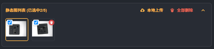
After uploading, all static images are displayed in the list. Users can perform the following operations:

Select Images: Check the images to use for workflow execution.
Delete Image: Remove the currently selected static image.
Delete All: Clear all current static image files.

Deletion is irreversible. Please proceed with caution.

When the workflow is executed and the node image source is set to "Static Image" mode,

the system uses the checked images from the static image list for task processing.

The platform supports selecting up to 5 static images simultaneously. The workflow uses these images sequentially as input sources for execution.

Multiple Image Sources

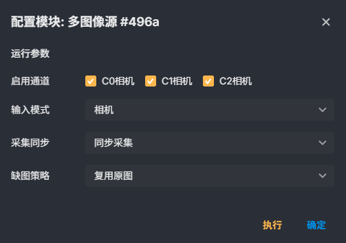
The Multiple Image Sources module obtains image data from multiple physical cameras at the same time. It supports configuring multiple camera channels and, according to the specified acquisition method and missing-image policy, provides stable multi-channel image input for subsequent vision processing flows. It is commonly used in scenarios such as multi-view inspection and parallel processing at multiple stations.

How It Works

The module opens the corresponding camera device or image stream entry point according to the configured camera identifier list (enabled channels).
On each triggered acquisition, the module acquires images from all enabled channels in parallel according to the configured acquisition method. Currently, only synchronous acquisition is supported, that is, all cameras capture one frame at the same moment.
If a channel fails to acquire an image because the camera is disconnected, a frame is dropped, or for other reasons, the module handles it according to the missing-image policy: for example, it reuses the last successfully acquired image, so that downstream modules always receive the agreed number of images and the flow is not interrupted by an abnormal individual camera.

Parameters

Parameter	Description	Default Value
Enabled Channels	Specifies the list of camera identifiers whose images need to be acquired. Each identifier corresponds to a physical camera or image stream entry point.	Empty (must be configured manually)
Acquisition Method	Sets the acquisition trigger mode of the cameras. Currently only "Synchronous Acquisition" is supported, which captures from all channels at the same time.	0 (Synchronous Acquisition)
Input Mode	Selects the source type of the image data. Currently only "Camera Input" is supported, that is, images are obtained from physical cameras.	0 (Camera Input)
Missing-Image Policy	The handling policy adopted when acquisition fails on a channel. The available option is "Reuse Previous Frame", which uses the last successfully acquired image to fill the channel that is missing in the current round, ensuring that the number of output images matches the number of channels.	0 (Reuse Previous Frame)

Camera Identifiers Must Be Accurate: The names entered in Enabled Channels must exactly match the camera IDs actually connected to the system; otherwise the corresponding channel cannot be opened successfully.
Channel Order Affects the Output: Downstream modules reference the images in the order of the enabled channel list. Before changing the order, confirm whether the subsequent processing logic still matches.
Choosing the Missing-Image Policy: If some cameras may occasionally drop frames, keep the "Reuse Previous Frame" policy to prevent the flow from being interrupted by missing images; if real-time images are required, monitor the image timestamps through external logic.
Only Synchronous Mode Is Currently Supported: All cameras are acquired at the same time by hard trigger or soft trigger, and the acquisition timing of each camera cannot be set individually. Make sure that the trigger signal can cover all cameras.
Resource Usage Considerations: When many high-resolution cameras are enabled, confirm that the processing capability and bandwidth of the host computer meet the requirements, to avoid acquisition delays or dropped frames caused by an excessive data volume.

Output Image

Overview

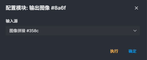
The Output Image module outputs the acquired image data in a vision flow. It connects the image acquisition stage with the subsequent processing, display, or storage stage, and steadily provides the images obtained by the camera or acquisition device to downstream use.

How It Works

After the upstream acquisition device finishes capturing an image, it sends the image data to the Output Image module. The module caches the image data and organizes the format, and passes it to downstream modules according to the connections in the flow. It mainly ensures that the image data reaches the next processing stage completely and continuously; the module itself does not perform image processing tasks such as recognition, measurement, or enhancement.

Use Cases

When the image captured by the camera needs to be passed to algorithm modules such as inspection, localization, and recognition.
When the acquired image needs to be displayed on the run interface for operators to observe.
When the acquired image needs to be saved or forwarded to an external system.

Light Source

Overview

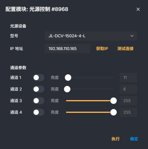
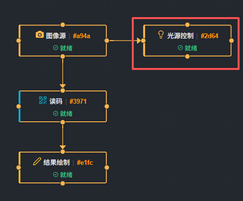
The "Light Source" module connects to and configures an external light source controller. Through this module, you can set the IP address and model of the light source controller and separately control the brightness and on/off status of 1~4 channels. The module also provides a light source connection test function, which makes it easy to confirm whether device communication is normal before formal operation.

In machine vision projects, the light source is a key factor affecting imaging quality. This module is suitable for scenarios that require unified management of light source controller parameters, per-channel light source adjustment, or verification of light source device connectivity.

How It Works

The module establishes communication with the light source controller according to the configured device IP address and light source model. After configuration is complete, you can choose "Set Light Source" or "Test Light Source Connection" as needed.

When "Set Light Source" is selected, the module sends the currently configured channel enable status and brightness values to the light source controller, so that each channel outputs according to the set parameters. When "Test Light Source Connection" is selected, the module tries to establish a connection with the light source controller at the specified IP address and returns the result of whether the connection succeeded.

Channel configuration supports 1~4 channels. Whether each channel is enabled and how bright it is can be set independently, which facilitates zone control in multi-channel light source systems. A channel that is not enabled outputs no light, and an enabled channel adjusts its luminous intensity according to the brightness value.

Use Cases

During device commissioning, verify whether the network connection between the host computer and the light source controller is normal.
In vision inspection tasks, when the light source brightness needs to be adjusted, or the light source state needs to be switched between different inspection items.
When using a multi-channel light source, control the on/off status and brightness of different channels separately to meet local lighting requirements.
When the light source controller model is JL-DCV-15024-4-L, configure the device parameters centrally through the module.

Parameters

Parameter	Description	Default Value
Device IP	The IP address of the light source controller. The module establishes network communication with the light source controller through this address.	No fixed default value; fill it in according to the actual device
Light Source Model	Select the model of the light source controller to be connected. The currently available model is JL-DCV-15024-4-L.	No fixed default value
Channel	Specifies the number of the light source channel to configure. Value range 1~4. Multi-channel light sources can be configured separately.	No fixed default value
Enable	Controls whether the current channel is enabled. Only an enabled channel outputs light, and a disabled channel does not emit light.	Disabled by default
Brightness	Sets the luminous brightness of the current channel. Value range 0~255; the larger the value, the brighter the light source, and 0 means the dimmest.	255

Steps

Add a "Light Source" module to the flow.
In the parameter configuration area, fill in the IP address of the light source controller.
Select the light source model according to the actual device.
Configure each channel that needs to be used: select the channel number, and set the enable state and the brightness value.
Select the "Operation Type". If the parameters need to be delivered to the light source controller, select "Set Light Source"; if you only need to verify whether the communication is normal, select "Test Light Source Connection".
Run the module and confirm whether the configuration succeeded according to the execution result.

Notes

Before entering the device IP, confirm that the light source controller and the host running Smart Vision Studio are reachable over the network; otherwise, the setting or the test may fail.
Only channels with "Enable" turned on output light. Even if a brightness value is set, a channel whose enable is not turned on still does not emit light.
The brightness value must be within the range 0~255. A value outside this range may cause the parameter delivery to fail or the light source controller to work abnormally.
The channel number range is 1~4. Configure it according to the actual number of channels on the light source controller and the wiring situation.
If you only need to confirm the communication status, select "Test Light Source Connection"; this operation does not change the current light output.

FAQ

Q: Why is the light source not lit even though a brightness value has been set?

A: First check whether the "Enable" of that channel is turned on. A channel whose enable is not turned on does not output light even if a brightness value is set. Next, confirm that the device IP and the light source model are correct, and that the light source controller is powered on and has finished the network connection.

Q: How can I tell whether the light source controller can be accessed normally?

A: Set the "Operation Type" to "Test Light Source Connection" and then run the module. If the execution result shows success, the current host can normally connect to the light source controller at the specified IP; if it fails, check the network connection, the IP address, and the power state of the controller.

Q: How many channels does the module support?

A: It supports 1~4 channels, and each channel can be set to its own enable state and brightness value.

Q: What brightness value is appropriate?

A: The brightness value range is 0~255, and the default value is 255. In actual use, adjust it according to the surface reflection of the object being measured, the camera exposure, and the ambient light conditions. It is recommended to start from a low brightness and increase it gradually to avoid overexposure of the image.

Image Processing

Image Processing is the process of preprocessing target images. When images have much interference or indistinct features, consider using image processing modules for preprocessing.

Filtering

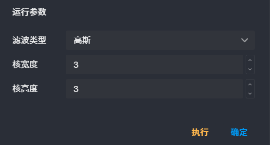
Filtering is a class of image processing algorithms. This module supports three filter types: Gaussian Filtering, Mean Filtering, and Median Filtering.

Gaussian Filtering
Gaussian filtering is a smoothing method based on the Gaussian function. Unlike mean filtering, Gaussian filtering assigns higher weights to center pixels and lower weights to edge pixels when calculating pixel averages. Gaussian filtering removes noise while better preserving image edge information.
- Parameters: filter kernel width and kernel height, value range 1~51. Larger values produce a more pronounced defocus effect, i.e., more blurred images.
- Suitable Scenarios: Gaussian filtering is suitable for removing Gaussian noise from images and performs well at preserving image edge information.
Mean Filtering
Mean filtering is one of the simplest smoothing methods. The principle of mean filtering is to replace each pixel value in the image with the average of its surrounding pixels. Mean filtering effectively removes noise but may cause the image to become blurry.
- Parameters: filter kernel width and kernel height, value range 1~51. Larger values produce a more pronounced defocus effect, i.e., more blurred images.
- Suitable Scenarios: Mean filtering is suitable for removing random noise from images but may blur image edges.
Median Filtering
Median filtering is a non-linear smoothing method. Its principle is to replace each pixel value in the image with the median of its surrounding pixels. Median filtering is very effective at removing salt-and-pepper noise (random black and white dots in images).
- Parameters: Filter kernel, value range 1~51. Larger values produce a more pronounced defocus effect, i.e., more blurred images.
- Suitable Scenarios: Median filtering is suitable for removing salt-and-pepper noise from images and performs well at preserving image edge information.

Morphological Processing

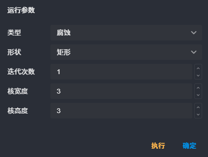
Through operations such as erosion, dilation, opening, and closing, effects such as noise removal, object separation, and edge detection on the image can be achieved. This module helps better process and analyze image data.

Morphological Types
- Dilation
  Dilation is the opposite of erosion - it is a process of expanding foreground objects in an image.
  Dilation convolves a structuring element with the image; as long as the structuring element overlaps with any foreground pixel in the image, the center pixel is preserved.
- Erosion
  Erosion is a process of shrinking foreground objects in an image.
  Erosion convolves a structuring element with the image; only when the structuring element completely covers the foreground pixels in the image is the center pixel preserved; otherwise, it is eroded away.
- Opening
  Opening is a combined operation of erosion followed by dilation.
  Opening is mainly used to remove small noise from images or separate connected objects.
- Closing
  Closing is a combined operation of dilation followed by erosion.
  Closing is mainly used to fill small holes in foreground objects or to connect broken objects.
Shape
Refers to the shape of the filter kernel, including Rectangle, Ellipse, and Cross.
Iterations
Refers to the number of operations performed on the original image in one morphological processing pass. More iterations produce a more noticeable effect. Value range: 1~10.
Kernel Width and Kernel Height
Value range 1~51. Increasing this value makes the effect of morphological processing more noticeable.

Binarization

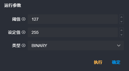
Image binarization converts the original image into an image containing only two grayscale values, 0 and 255. The purpose of binarization is to simplify the image, highlight target contours, and facilitate subsequent image processing. A binarized image helps the algorithm identify edges and features in the image more accurately.

Type
- BINARY
  That is, binarization: values greater than the threshold become the maximum value, and values less than the threshold become 0.
- BINARY_INV
  That is, inverse binarization: values greater than the threshold become 0, and values less than the threshold become the maximum value.
- TRUNC
  That is, truncation: values greater than the threshold become the threshold, and values less than the threshold remain unchanged.
- TOZERO - To Zero
  That is, to zero: values greater than the threshold remain unchanged, and values less than the threshold become 0.
- TOZERO_INV
  That is, inverse to zero: values greater than the threshold become 0, and values less than the threshold remain unchanged.
Threshold
Threshold, used to segment the pixel values of an image.
Set Value
If a pixel value is greater than the threshold, it is set to this value (usually 255).

Image Scaling

Image scaling adjusts the original image to a specified width and height. Its main purpose is to unify the input size, reduce the amount of computation, or adapt to subsequent algorithms (such as model input and display windows).

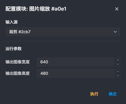
Runtime Parameters

Output Image Width: Specifies the width of the scaled image (unit: pixel).
Output Image Height: Specifies the height of the scaled image (unit: pixel).

Geometric Transformation

Geometric transformation adjusts the spatial structure of an image, including operations such as mirroring and rotation. Such operations do not change the pixel values themselves, but change the positional relationship of the pixels. They are commonly used for image orientation correction, data augmentation, or adapting to subsequent processing flows.

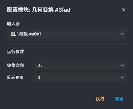
Runtime Parameters

Mirror Direction: Controls whether flipping is performed and the flipping method:
- None: No mirroring is performed
- Horizontal: Flips along the horizontal direction (left-right mirror)
- Vertical: Flips along the vertical direction (top-bottom mirror)
- Horizontal and Vertical: Performs horizontal and vertical flipping at the same time (equivalent to rotating 180°)
Rotation Angle: Controls the image rotation angle. Supports fixed angles or custom input:
- 0°: No rotation
- 90°: Rotates 90 degrees clockwise
- 180°: Rotates 180 degrees
- 270°: Rotates 270 degrees clockwise
- Custom: Rotates by the specified angle (unit: degree)

Image Stitching

The Image Stitching module combines multiple input images into a single image according to a specified arrangement. It is commonly used in scenarios that require side-by-side display, comparative analysis, or stitching of consecutive frames, and can quickly generate a seamless combined image in the horizontal or vertical direction.

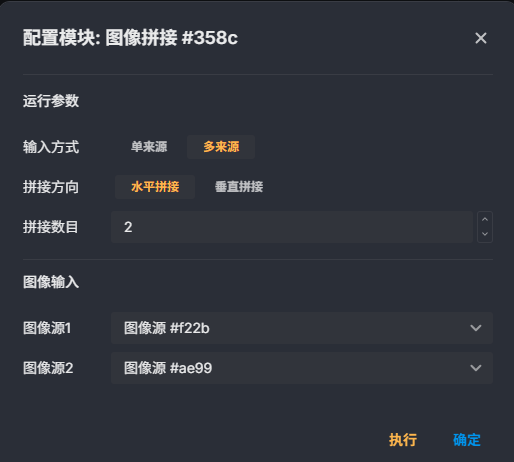
How It Works

The module receives a set of images passed in from upstream nodes (at least two).
Determines the arrangement direction according to the stitching method selected by the user:
- Horizontal stitching: all images keep the same height and are placed in order from left to right.
- Vertical stitching: all images keep the same width and are placed in order from top to bottom.
If the input images differ in size, the module automatically aligns them based on the size of the first image (the remaining images may be stretched or cropped), and finally outputs a complete combined image.

Parameters

Parameter	Description	Default Value
Stitching Method	Select the arrangement direction of the images: • Horizontal stitching — images are arranged from left to right in the horizontal direction • Vertical stitching — images are arranged from top to bottom in the vertical direction	Horizontal stitching

To ensure a good stitching result, it is recommended to keep the input images at a uniform size; if the sizes are inconsistent, the module aligns them based on the first image, which may deform or lose part of the image content.
The stitching direction directly affects the output layout. Select horizontal or vertical according to the final display requirement.
When there are many input images, the pixel size of the output image increases multiplicatively and may consume a lot of memory. It is recommended to estimate the resource usage in advance.
The module itself does not provide spacing or border settings between images. If margins are required, use modules such as "Image Crop" or "Canvas Extension" together.

Image Enhancement

The Image Enhancement module improves image quality, increases the distinction between the target and the background, and provides clearer input for subsequent detection, recognition, or measurement.

This module provides processing methods such as sharpening, contrast adjustment, Gamma correction, and brightness correction. It effectively handles problems such as blurred image edges, insufficient contrast, uneven illumination, or an overall image that is too dark or too bright. Users can select one or more enhancement operations according to the actual image conditions and flexibly adjust the parameters to make image features more prominent.

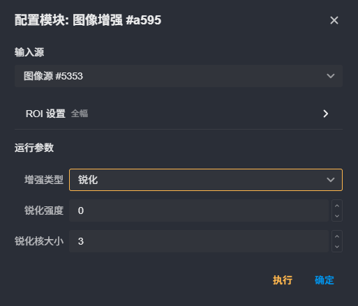
How It Works

The module receives one or more input images and allows specifying a region of interest (ROI). According to the enhancement type selected by the user, the module processes the image at the pixel level:

Sharpening: Strengthens areas in the image where grayscale changes sharply, making edges and details clearer. The sharpening strength and kernel size together determine the degree and scope of the enhancement.
Contrast Adjustment: Changes the dynamic range of the image grayscale through a contrast coefficient, making bright areas brighter and dark areas darker, thereby enhancing the difference between the target and the background.
Gamma Correction: Compensates the overall brightness of the image using a non-linear mapping. It mainly affects the mid-gray region while preserving details in bright and dark areas.
Brightness Correction: Linearly adjusts the overall brightness of the image through brightness compensation and gain. It is suitable for scenes that are overall too dark or too bright.

After processing is complete, the module outputs the enhanced image for use by other modules in subsequent flows.

Use Cases

When uneven lighting makes part of the image too dark or too bright, use brightness correction to compensate for the brightness difference.
When the overall contrast of the image is low and the target is difficult to distinguish from the background, use contrast adjustment to enhance the difference.
When image edges are blurred and details are unclear, use sharpening to highlight edges and textures.
When the non-linear response of the imaging system or the display device needs to be corrected, use Gamma correction to improve the visual effect.

Parameters

Parameter	Description	Default Value
Image Enhancement Type	Selects the image enhancement method. Options: "Sharpen", "Contrast", "Gamma", "Brightness Correction". After selection, the interface displays the corresponding parameters for adjustment.	Sharpen
Sharpening Strength	Controls the strength of the sharpening effect. The larger the value, the more obvious the edge enhancement, but an excessively high value may amplify noise. Takes effect only for the "Sharpen" type. Value range 0~100.	0
Sharpening Kernel Size	Sets the size of the neighborhood window used for sharpening, which must be an odd number. The larger the kernel, the wider the sharpening range, but an excessively large kernel may cause loss of detail or increase processing time. Takes effect only for the "Sharpen" type. Value range 1~51.	3
Contrast Factor	Adjusts the image contrast. A value greater than 100 enhances the contrast, and a value less than 100 reduces the contrast. Value range 1~10000.	100
Gamma	Sets the Gamma correction value. A value greater than 1 brightens the whole image, and a value less than 1 darkens the whole image. Keep two decimal places. Range 0.00~10.00.	1.00
Brightness Correction Compensation	Adds to or subtracts from the overall image brightness during brightness correction. A positive value brightens the image, and a negative value darkens it. Value range -255~255.	0
Gain	Works together with Brightness Correction Compensation to adjust the gain amplitude of brightness correction. Value range 0~100.	0

Notes

An excessively high sharpening strength amplifies noise in the image. Start from a lower value and adjust gradually to find the balance between edge enhancement and noise suppression.
The sharpening kernel size must be an odd number. If it is too large, image details may be lost or the computation time may increase significantly.
Gamma correction and brightness correction both affect the overall image brightness. Avoid using them at the same time, which may cause overexposure or underexposure.
If the contrast factor deviates too far from 100, details in bright or dark areas may saturate. Adjust it according to the actual image.
If an ROI area is set, only pixels inside the area are processed and the area outside remains unchanged. Confirm whether the ROI range covers the target area.

Color Processing

Color Conversion

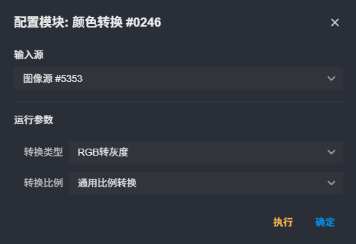
The Color Conversion module converts the color space of an image. It supports converting an RGB color image into a grayscale, HSV, HSI, or YUV image.

It is suitable for preprocessing steps that need to extract brightness, color, or chrominance information, and helps subsequent detection algorithms obtain more stable and easier-to-analyze image input.

How It Works

The module receives a color image. When the conversion type is set to "RGB to Grayscale", the module combines the R, G, and B channels into a single-channel grayscale image according to the configured conversion ratio. The conversion ratio can use the average method, take the maximum or minimum channel value, directly use one channel, or perform weighted calculation based on the R, G, and B coefficients set by the user.

When the conversion type is set to HSV, HSI, or YUV, the module converts the image from the RGB color space to the target color space and obtains a multi-channel result. In this case, you can select the first channel, second channel, or third channel to view through the Display Channel parameter. The final output is the converted image, which is used by subsequent flows.

Parameters

Parameter	Description	Default Value
Conversion Type	Selects the target type of color space conversion. Options: "RGB to Grayscale", "RGB to HSV", "RGB to HSI", "RGB to YUV". This parameter determines the parameters that can be configured afterwards and the type of the output image.	RGB to Grayscale
Conversion Ratio	Visible only when the conversion type is "RGB to Grayscale". Determines how the R, G, and B channels are combined when calculating grayscale. Options: "General Ratio Conversion", "Average Ratio Conversion", "Channel Minimum", "Channel Maximum", "Custom Ratio Conversion", "R Channel", "B Channel", "G Channel", "Unconstrained Ratio Conversion". Different methods affect the brightness and contrast performance of the grayscale image.	General Ratio Conversion
Display Channel	Visible when the conversion type is HSV, HSI, or YUV. Selects the single-channel image to display in the conversion result. Options: "First Channel", "Second Channel", "Third Channel".	First Channel
R Channel Coefficient	Used when the conversion ratio is set to "Custom Ratio Conversion" to set the weight of the R channel in the grayscale calculation. Adjust it reasonably according to the actual image and the detection target.	No default value
G Channel Coefficient	Used when the conversion ratio is set to "Custom Ratio Conversion" to set the weight of the G channel in the grayscale calculation. Adjust it reasonably according to the actual image and the detection target.	No default value
B Channel Coefficient	Used when the conversion ratio is set to "Custom Ratio Conversion" to set the weight of the B channel in the grayscale calculation. Adjust it reasonably according to the actual image and the detection target.	No default value

Notes

The conversion ratio parameter appears only for RGB to Grayscale. It does not need to be configured when converting to HSV, HSI, or YUV.
Non-grayscale conversion results contain multiple channels. To view a single channel, switch it through Display Channel. Avoid directly observing the color composite result, which may lead to misjudgment.
When Custom Ratio Conversion is selected, set the R, G, and B coefficients according to the image content and the detection target. Inappropriate weights may reduce the contrast between the target and the background.
Channels have different meanings in different color spaces. Confirm the information corresponding to the required channel before use.

Localization and Target Extraction

Crop

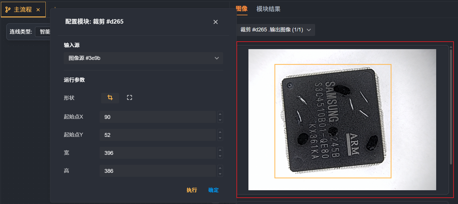
Cropping is the process of removing all unwanted areas from an image, or highlighting a specific feature of the image.

Parameter Configuration
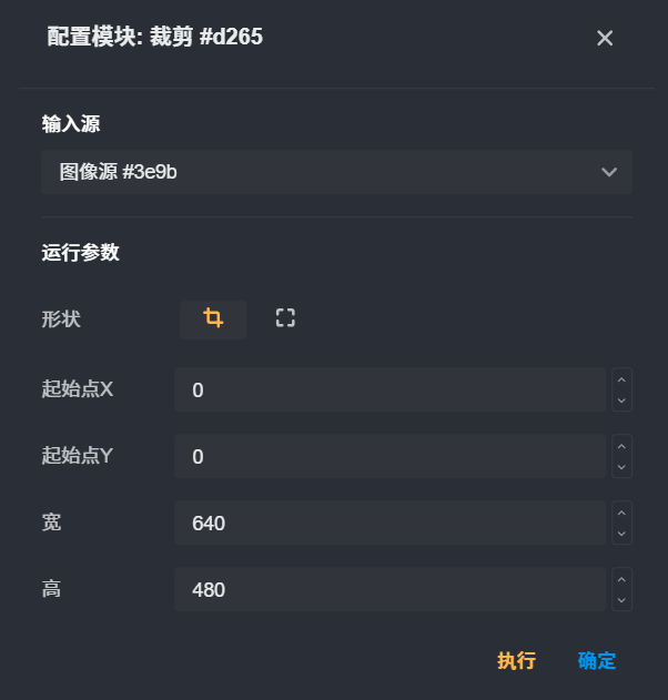
- Input Source: Generally the output image of the Image Source module, or the output image of other image processing category modules.
- Shape: Two types: Rectangle and Full Frame.
  By default, the image-related parameters of the preceding module are displayed. You can draw a selection box directly in the image display area, and after selection fine-tune it with the up and down keys of the input fields. Click "Full Frame" to restore to the initial state. When the selection area meets the requirements, click "Execute" directly to view the result.

Contour Detection

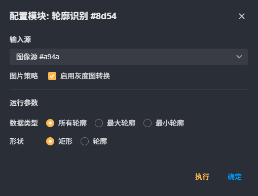
Contour Detection is used to extract the boundaries of objects in an image. It filters out target objects that meet the requirements through the configured Area and Length. It can be used for object recognition, shape analysis, target tracking, and other applications.

Basic Concepts
- Contour: The boundary of an object in an image, composed of a series of points.
- Contour Features: The area, perimeter, bounding rectangle, minimum bounding rectangle, minimum bounding circle, and other features of a contour.
Parameter Settings
- Data Type: Which contours to output. Options: "All Contours", "Largest Contour", or "Smallest Contour".
- Shape: The representation form of the output result. Options: Rectangle or Contour. Rectangle indicates the bounding rectangle area of the target, and Contour indicates the actual boundary shape of the target.
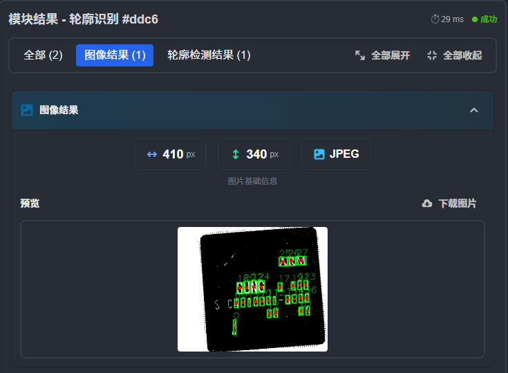
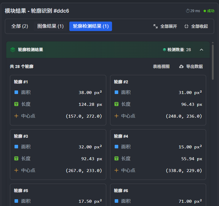
Module Results
The output results of this module include the number of qualified contours, and the area, length, and center point coordinates of each contour.
As shown below:

Blob Analysis

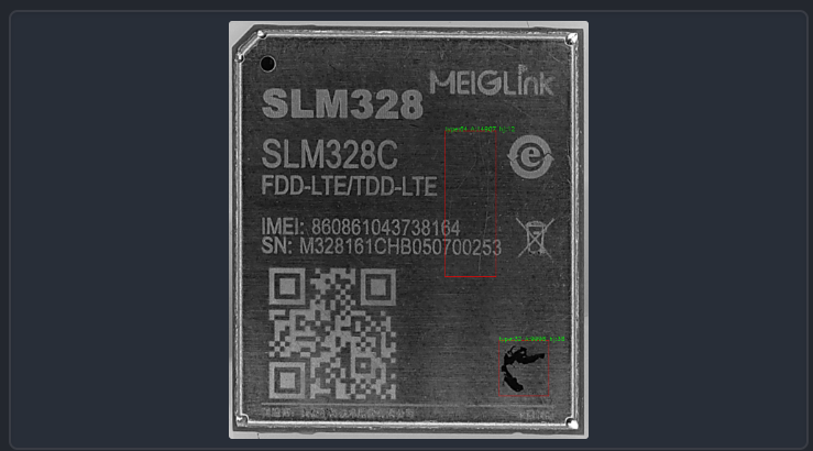
Blob Analysis is an image analysis tool in the Localization and Target Extraction category, used to detect and extract connected regions in an image. In actual inspection, when the target and the background can be distinguished by grayscale, color, or binarization results, Blob Analysis helps users quickly locate the area where the target is.

Through Blob Analysis, you can obtain information such as the area, position, and boundary of the target, so as to filter and judge the targets in the image.

A mask needs to be configured. The module preferentially searches for connected targets within the area limited by the mask; the common ones are Contour Detection, DL Localization, and DL Segmentation;

For the specific analysis range when no mask is configured, refer to the actual running results of the software.

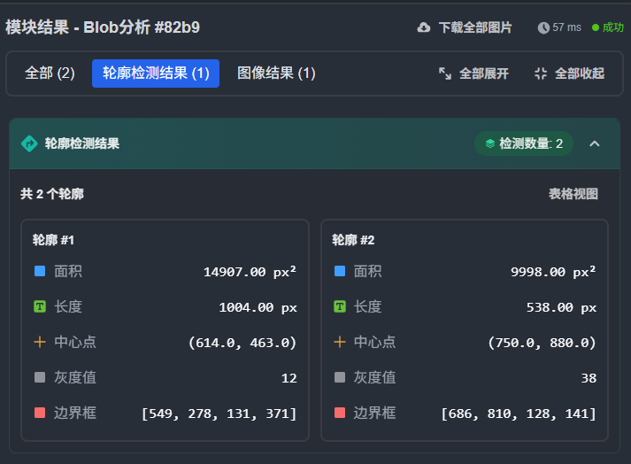
Common Output Information

Area: The number of pixels in the connected region
Length
Grayscale
Bounding Box: The minimum enclosing rectangle of the target
Centroid: The geometric center of the region

Contour Cropping

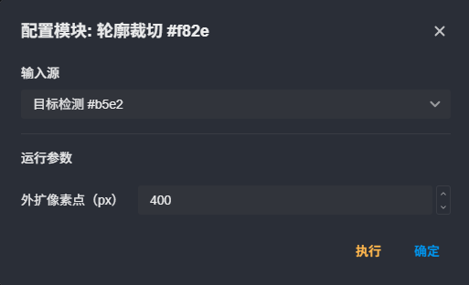
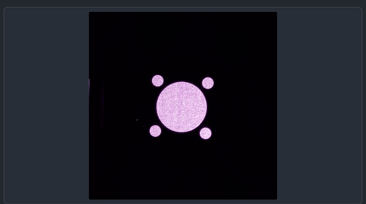
The Contour Cropping module is used to crop the target area in an image according to the target contour. It needs to work together with a deep learning model, receives the contour or mask information output by the model, automatically determines the target boundary, and expands the cropping range according to the configured expansion pixels, finally obtaining an image that contains only the target area. This module is suitable for scenarios where detection or segmentation results need to be separated from the original image, such as target object extraction and region of interest cropping.

How It Works

The Contour Cropping module runs as a post-processing step of the deep learning node. It receives the original image to be processed and the target contour or mask information output by the associated deep learning model, and determines the region corresponding to the target contour in the image. Users can set the expansion pixels so that the cropping boundary expands outward by a certain distance from the original contour, avoiding loss of target edge information. The module calculates the final cropping range based on the contour region and the expansion amount, and outputs the cropped image or region. The whole process is automatic; users only need to configure the associated deep learning node and the expansion parameter.

Parameters

Expansion pixels: Controls the pixel distance by which the cropping boundary expands outward from the target contour. Properly increasing this value prevents the target edge from being cropped off, but setting it too large may introduce too much background

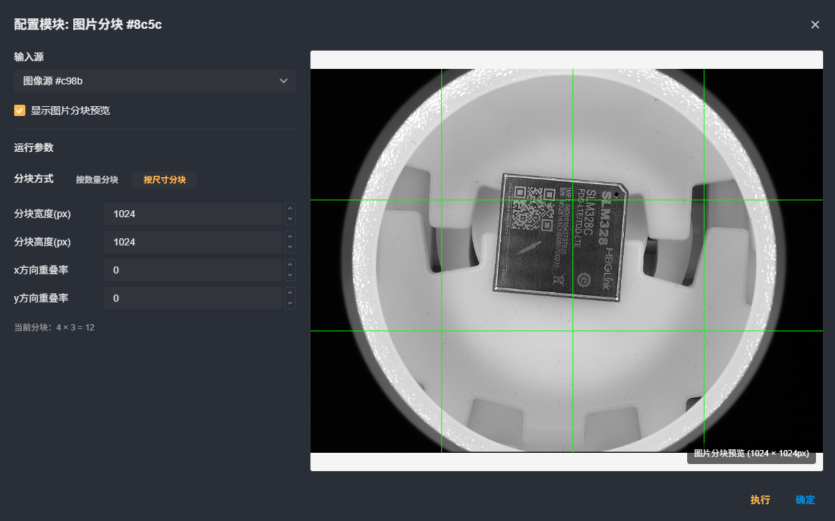
Image Blocking

Image Blocking is used to divide the input image into multiple rectangular regions according to a specified count or a specified size, so that subsequent localization, detection, or recognition modules can process them separately. When the image resolution is high, the target size is small, or the target distribution range is wide, processing the whole image directly tends to reduce detection accuracy or algorithm efficiency. Using this module, the image can be split into multiple local regions, making it convenient for subsequent flows to perform target extraction and analysis block by block.

How It Works

According to the configured blocking method and parameters, this module generates several rectangular block regions on the input image. In "By Count" mode, the module divides the image into several columns and rows along the corresponding directions according to the X-direction tile count and Y-direction tile count, forming a uniform grid; in "By Size" mode, the module uses the configured width and height as the basic unit and successively divides the image into tiles of a fixed pixel size. In either mode, the X-direction overlap rate and Y-direction overlap rate control the degree of overlap between adjacent tiles, avoiding missing targets that fall on block boundaries. Finally, the module outputs each block region for subsequent flow processing.

Use Cases

Small target detection on large-format images: Divide the whole image into multiple local regions to avoid small targets being ignored during scaling or global processing.
Localization and extraction when targets are widely distributed: Process different regions separately to reduce interference from invalid regions.
High-resolution image processing: Divide the image into several sub-images for batch processing to reduce the memory and computation pressure of a single processing run.
Scenarios prone to missed detection at edges: By setting the overlap rate, adjacent blocks have overlapping areas, reducing missed detection caused by targets being cut by block boundaries.

Parameters

Parameter	Description	Default Value
Blocking Method	Select the way to divide the image. Options: "By Count" or "By Size". In "By Count" mode, the image is evenly divided into the specified number of rows and columns; in "By Size" mode, each block has a fixed width and height.	By Count
X-direction Tile Count	In "By Count" mode, the number of divisions of the image in the horizontal direction. The larger the value, the finer the blocks in the horizontal direction and the smaller each block. Value range: 1~50.	1
Y-direction Tile Count	In "By Count" mode, the number of divisions of the image in the vertical direction. The larger the value, the finer the blocks in the vertical direction and the smaller each block. Value range: 1~50.	1
X-direction Overlap Rate	The overlap ratio of adjacent blocks in the horizontal direction. A larger overlap rate reduces missed detection when targets fall on horizontal block boundaries, but increases the number of blocks and subsequent processing load. Value range: 0~100.	0
Y-direction Overlap Rate	The overlap ratio of adjacent blocks in the vertical direction. A larger overlap rate reduces missed detection when targets fall on vertical block boundaries, but increases the number of blocks and subsequent processing load. Value range: 0~100.	0
Block Width	In "By Size" mode, the width of a single block, in pixels. Effective only when the blocking method is "By Size".	No default value; must be set in "By Size" mode
Block Height	In "By Size" mode, the height of a single block, in pixels. Effective only when the blocking method is "By Size".	No default value; must be set in "By Size" mode

Circle Finding

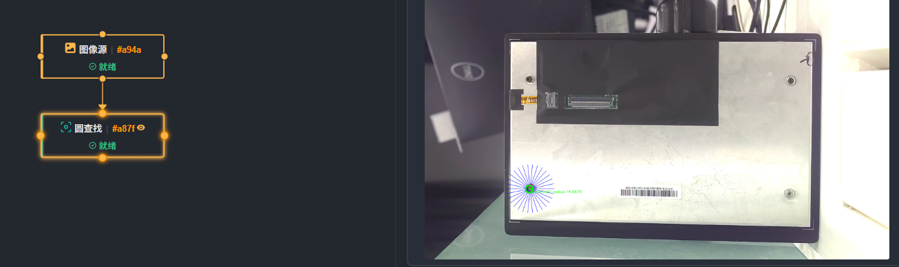
The Circle Finding module is used to quickly and accurately locate circular targets in an image; it belongs to the Localization and Target Extraction category of tools. It can recognize complete or partial circular contours and output geometric information such as the circle center coordinates and radius. When you need to detect the position and size of circular holes, circular parts, or ring-shaped features on a workpiece, this module can complete the localization automatically and work with subsequent tasks such as measurement or alignment.

How It Works

Within the specified annular search region, the module evenly places multiple calipers along the circumference, and each caliper extracts edge points matching the configured polarity along the radial direction. Then, a circle is fitted based on all valid edge points, outliers with large deviations are removed, and the circle center position and radius are finally obtained. To balance detection speed and accuracy, the initial localization mode can be enabled: first downsample the image for fast coarse localization, then perform precise localization at the original resolution. Parameters such as the edge threshold, edge polarity, and edge type control how edge points on the caliper are filtered, ensuring that only reliable contour points are included in the fitting calculation.

Use Cases

Localization and alignment of circular features on mechanical parts (such as locating holes and assembly holes).
Recognition of pads and circular mark points on electronic components.
Size measurement and appearance inspection of circular workpieces or products.
Pose confirmation of ring-shaped regions, for example, localization of the inner and outer rings of a bearing.

Parameters

Parameter	Description	Default Value
Sector Ring Radius	Defines the inner boundary radius of the annular search region. Narrowing the range reduces interference and improves speed, but make sure the edge of the circle to be measured is included.	10~100
Caliper Count	The number of radial calipers distributed on the circumference of the sector ring. The more calipers, the denser the detected edge points and the more stable the fitting, but the longer the processing time.	30
Edge Threshold	The contrast threshold for filtering edge points on the caliper, value range 0~255. Edges below this threshold are ignored. Raising the threshold suppresses noise, but weak edges may be missed.	15
Edge Polarity	Specifies the transition direction of the searched edge: black to white, white to black, or any polarity. Choose according to the brightness relationship between the target circle and the background.	Any Polarity
Edge Type	When multiple edge points on a caliper meet the conditions, determines which one to use: the strongest edge, the last edge, or the first edge.	Strongest
Initial Localization	When enabled, the module first downsamples the image for fast coarse circle finding, then performs precise localization on the original image. Suitable for scenes with a large field of view or large position offset.	Off
Downsampling Factor	The image scaling factor during initial localization. The higher the factor, the faster the speed, but the accuracy of coarse localization may decrease. Can be set only when Initial Localization is enabled.	8
Circle Localization Sensitivity	The sensitivity for determining whether a circle exists during the initial localization stage. The larger the value, the easier it is to detect, but false detection may also be introduced. Can be set only when Initial Localization is enabled.	10
Removal Count	The maximum number of outlier edge points allowed to be removed when fitting the circle. Properly increasing the removal count can eliminate errors caused by local occlusion or interference, but excessive removal may make the fitting result unstable.	0
Filter Size	The size of the smoothing filter applied to the image before detection, used to suppress noise while preserving edges and avoiding edge blur. Range: 1~50.	2

The annular search region should be as concentric with the target circle as possible, and the ring width only needs to contain the complete circumference; it should not be too wide, so as to avoid introducing irrelevant edges.
The edge threshold should not be set too low, otherwise noise or texture may be misjudged as edges, resulting in a wrong fitting.
When Initial Localization is enabled, the downsampling factor and circle localization sensitivity jointly affect the coarse localization result; a large factor is fast but may cause localization deviation, so it is recommended to start with the default values.
The caliper count affects processing time and fitting accuracy. For circles with a small radius, the caliper count can be reduced appropriately to improve efficiency.
When using the removal count function, make sure that the remaining edge points after removal can still fully cover the circumference; otherwise the fitting result may shift.

Edge Finding

The Edge Finding module is used to quickly locate the edge features of a target in an image. By setting the edge strength, polarity, and filtering method, it extracts edge points or edge segments that meet the conditions. This module is usually used in target localization and target extraction scenarios. It can stably find object boundaries in complex backgrounds and provide reliable position information for subsequent measurement, alignment, and inspection tasks.

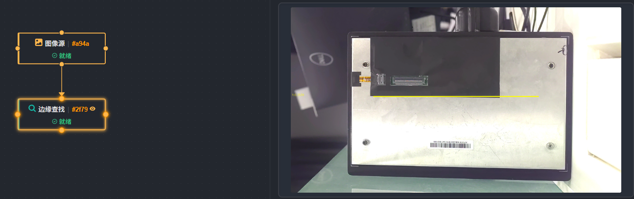
How It Works

Image Preprocessing: If the grayscale image option is enabled, first convert the input image to a grayscale image to reduce channel complexity and focus on brightness changes. Then apply smoothing filtering of the specified size to the image to suppress the interference of noise on edge detection.
Edge Detection and Threshold Filtering: Compute the gradient strength of each pixel on the preprocessed image to obtain an edge response map. According to the configured edge threshold, only pixels whose strength is higher than the threshold are regarded as candidate edge points. The candidate points can also be filtered by direction according to the edge polarity (black to white, white to black, or any polarity).
Edge Selection and Sorting: For candidate edges that pass the threshold and polarity filtering, control the number of output results according to the selected edge selection method (such as keep all, keep the strongest first N by strength, or take a specified number starting from the first candidate or from the last candidate). Finally, sort the results according to the configured sorting method (by score, by direction, etc.) and output the final edge list. In the localization and target extraction flow, the module is usually a preceding step of feature extraction, providing stable edge information for feature matching or geometric localization.

Parameters

Parameter	Description	Default Value
Enable Grayscale Image	Whether to convert the input image to grayscale before edge detection. If the input is already grayscale, it is recommended to keep it enabled to improve computation efficiency.	On
Filter Size	The size of the smoothing filter applied to the image before edge detection. The larger the value, the stronger the noise reduction, but edge details may be lost or shifted. Value range 1~51.	-
Edge Threshold	The threshold that controls edge detection sensitivity. Only pixels with gradient strength higher than this value are regarded as edge candidates. Value range 0~255. The lower the threshold, the more edges are detected; the higher the threshold, the more only strong edges are kept.	-
Edge Polarity	Select the brightness change direction of the edge to be detected: any polarity, black to white (dark area to bright area), or white to black (bright area to dark area). It can be set according to the actual appearance direction of the target edge, which helps filter background interference.	Any Polarity
Edge Selection Method	The retention strategy for candidate edges: keep all edges; keep the strongest first N by strength; take the first N starting from the first detected edge; or take the first N starting from the last edge. Combined with the maximum result count, the output quantity can be finely controlled.	All
Maximum Result Count	The maximum number of edges finally output, value range 1~1000. This value takes effect only when the edge selection method is not "All", and is used to limit the number of selected edges.	-
Sorting Method	The basis for sorting the output edges: by strength score in descending or ascending order, or by edge direction in forward or reverse order. The sorting result affects the order of subsequent feature matching and may affect matching speed and accuracy.	Score Descending

Balance Between Filter Size and Localization Accuracy: The larger the filter size, the edge localization may be shifted by smoothing. For high-precision localization scenarios, it is recommended to use a smaller filter size (such as 3) together with appropriate lighting and image preprocessing to reduce noise.
Adjust the Edge Threshold According to the Actual Image: If the image contrast is low, lower the threshold appropriately to detect more edges; if there is much background texture or interference, raise the threshold to keep only significant edges and avoid false detection.
Polarity Selection Can Greatly Reduce False Edges: When the brightness transition direction of the target is known (for example, a dark object on a bright background), selecting the corresponding polarity (such as white to black) can shield the opposite edges and improve detection reliability.
Use the Selection Method Together with the Maximum Result Count: The "Maximum Result Count" only affects the filtering process when the "Edge Selection Method" is not "All". If you want to get all edges, keep the selection method as "All"; in this case the maximum result count has no effect.
Sorting Method Affects Subsequent Localization: If the edge results will be used for shape-based matching or line fitting, sorting by direction may help subsequent algorithms obtain a more stable feature sequence.

Line Finding

The Line Finding module is used to quickly and accurately locate straight-line edges in an image and output the position and direction information of the line. It automatically extracts edge points and fits a line by placing multiple sets of calipers along the search region. It is suitable for scenarios such as workpiece localization, angle measurement, and edge-guided alignment. When high-precision localization or measurement based on a line feature is required, this module can be selected.

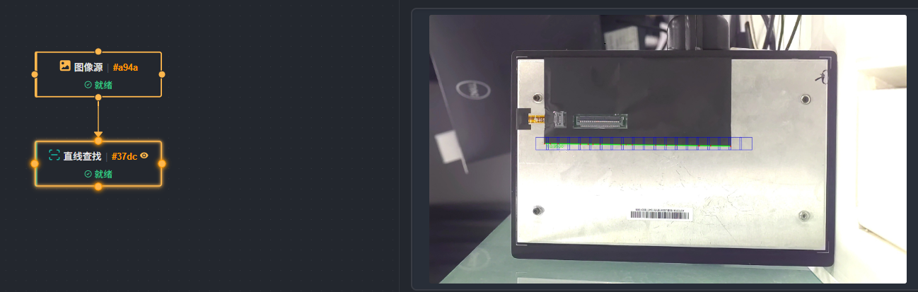
How It Works

The module first applies smoothing filtering to the input image to reduce the interference of noise on edge extraction. Then, within the user-defined region of interest (ROI), several calipers are evenly placed perpendicular to the expected direction, and one candidate edge point is extracted in each caliper according to the configured edge polarity and threshold. After obvious outliers are removed, a straight line is fitted to the remaining valid points using the least squares method. If the angle constraint is enabled, the module further filters on the basis of the fitting according to the expected angle and rotation tolerance range; finally it outputs the line information that meets the conditions, including the center coordinates, angle, start point, and end point.

Use Cases

Workpiece Edge Localization: Use the product edge line as the reference to obtain the position and pose of the workpiece for subsequent picking or assembly.
Angle Measurement: Detect the included angle of a part edge relative to a reference line to judge installation or machining deviations.
Guided Alignment: In a vision guidance system, use the detected line as the alignment reference to drive robot motion.
Quality Inspection: Determine whether a product edge is straight and whether it has defects or burrs.

Parameters

Parameter	Description	Default Value
Filter Size	The size of the convolution kernel used to smooth and filter the image, suppressing the interference of noise on edge detection. The larger the value, the blurrier the image and the more suitable it is for images with a low signal-to-noise ratio, but it reduces localization accuracy.	2
Number of Calipers	The total number of calipers placed along the search direction. The more calipers, the denser the edge points involved in the fitting and the more reliable the fitting result, but the longer the processing time.	20
Edge Polarity	Specifies the direction of the brightness change of the detected edge. Options: "Black-to-White", "White-to-Black", or "Any Polarity". Selecting the correct polarity extracts only the target edge and avoids interference.	Any Polarity
Edge Threshold	The minimum contrast for edge point detection, with a value range of 1-255. Only points whose grayscale change amplitude is greater than this threshold are treated as candidate edge points. Increasing the threshold suppresses weak edges and noise, but may lose the target edge.	15
Edge Type	When multiple edges satisfying the conditions exist in the same caliper, determines which point participates in the fitting. Options: "Strongest", "Last", "First", or "Near Centerline". "Strongest" selects the edge with the highest contrast, "First" and "Last" are ordered by the search direction, and "Near Centerline" selects the edge close to the caliper centerline.	Strongest
Number of Rejected Points	The number of outliers allowed to be rejected before fitting the line. When some edge points deviate from the line due to interference, an appropriate rejection value excludes the abnormal points and improves fitting robustness.	0
Angle Enable	Whether to enable the angle constraint. When enabled, only lines whose angle is near the expected angle and whose deviation is within the rotation tolerance are accepted; when disabled, the fitting result in any direction is output.	Off
Expected Line Angle	When "Angle Enable" is enabled, sets the expected angle (in degrees) of the target line. The module preferentially searches for lines close to this angle.	0.00
Angle Rotation Tolerance	When "Angle Enable" is enabled, the maximum deviation allowed for the line angle relative to the expected angle. A larger value accommodates slight workpiece deflection, while a smaller value filters out interfering lines with large direction differences.	180.00
Angle Normalization	Whether to normalize the detected line angle to a specific range (usually [-180°, 180°]). When enabled, the output angle is mapped into this range for unified subsequent processing.	Off
Line Finding Reverse	Whether to reverse the start point and end point direction of the line. Enable this option when the vector direction of the line must be unified to meet specific flow requirements.	Off

Try to make the drawing direction of the ROI perpendicular to the target line so that the calipers can effectively intercept edge changes and improve the quality of edge point extraction.
More calipers is not necessarily better. Overly dense calipers increase the computation time and provide limited accuracy improvement. Set the number moderately according to the ROI length and edge quality.
When the image noise is high, first increase the filter size and the edge threshold appropriately. After stable results are obtained, optimize gradually to balance accuracy.
After the angle constraint is enabled, if the tolerance range is set too small, the finding may fail due to slight workpiece deflection. In this case, relax the tolerance value appropriately.
The number of rejected points should not be too large, otherwise normal edge points may be rejected as outliers, which instead reduces the fitting accuracy. It is usually recommended not to exceed 5% of the number of calipers.

Position Correction

The Position Correction module performs a spatial transformation on the preceding localization results to convert the detected target position and angle into a specified reference coordinate system. Typical scenarios include: mapping the matching result in the pixel coordinate system to the world coordinate system, or uniformly compensating for localization deviations between multiple processes. Use this module when you need to adjust the reference origin or rotation angle of the localization result, or to align datum points.

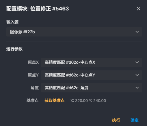
How It Works

The module receives the detection points, angles, and other information generated by the preceding localization tool (such as template matching or circle finding), and performs coordinate transformation according to the set correction method. When the "By Point" method is selected, the module automatically calculates the offset and the rotation angle according to the correspondence between the datum point coordinates defined by the user (usually the theoretical coordinates of two or more points) and the current measured values, completing the position calibration. If the "By Coordinate" method is selected, the module directly uses the X/Y offset and rotation angle entered by the user to translate and rotate the localization result. After processing, the output coordinates and angle are the corrected results, and subsequent measurement or localization steps can be based on this corrected coordinate system.

Use Cases

Before high-precision alignment and placement, use datum mark points to correct the global offset and rotation of visual localization.
When the equipment has mechanical vibration or installation errors, periodically correct the deviation between the image coordinate system and the mechanical coordinate system through calibration points.
After template matching, redefine the measurement origin to simplify the coordinate calculation of subsequent measurements.

Parameters

Parameter	Description	Default Value
Origin X	Sets the X coordinate offset of the origin of the corrected coordinate system. This value is added to the X coordinate of the current localization result to achieve translation.	-
Origin Y	Sets the Y coordinate offset of the origin of the corrected coordinate system. This value is added to the Y coordinate of the current localization result to achieve translation.	-
Angle	When the method is set to "By Coordinate", sets the rotation angle of the coordinate system (unit: degree). A positive value indicates counterclockwise rotation, and a negative value indicates clockwise rotation.	-

The By Point method requires a one-to-one correspondence between datum points and actual detection points, and the number of points must not be less than 2; otherwise, a complete spatial transformation cannot be calculated.
The input offset and angle are calculated based on the current localization result. Pay attention to the sign direction to avoid reversing the direction of the coordinate system after correction.
The angle unit is degree, and the input range is usually -360° to 360°. If it exceeds this range, the module may normalize it automatically.
When the By Point method is selected, the datum point coordinates should be theoretical values (the ideal positions in the target coordinate system), not the pixel coordinates in the actual image.
If the preceding localization result is unstable, the output of position correction fluctuates accordingly. Ensure the stability of the localization module first.

Caliper Tool

The Caliper Tool is used to locate an edge or an edge pair in an image and is a common tool in machine vision measurement and localization. It can scan grayscale changes along a set direction within a specified detection area, find edge points that meet the strength and polarity requirements, and output information such as the edge position and score. Use the Caliper Tool when a task requires measuring workpiece width, locating an edge position, detecting a gap, or counting edge structures.

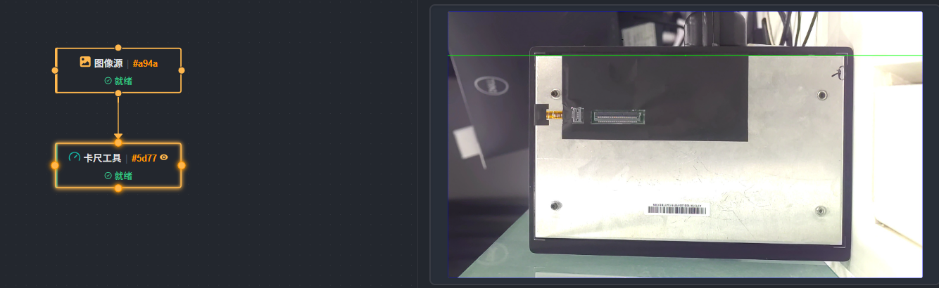
How It Works

Within the specified detection area, the Caliper Tool first performs grayscale projection on the image along the caliper length direction to obtain a grayscale change curve. It then smooths the curve according to the set filter size to reduce the interference of image noise on edge localization. The tool calculates the edge strength on the smoothed curve and screens out candidate edge points according to the edge threshold.

Among the candidate edges, the tool further determines whether the grayscale change direction meets the requirements according to the edge polarity. For single edge mode, the tool directly outputs one or more edges that meet the conditions; for edge pair mode, the tool searches for two edges that satisfy the width constraint according to the set edge pair width range, forming an edge pair result.

When multiple results are detected, the tool arranges the results according to the sorting method and outputs them according to the maximum number of results. The curve feature parameters define the physical meaning and value range of the edge scoring curve and help the tool screen or sort edges by features such as contrast, grayscale, position, and spacing.

Parameters

Basic Parameters

Parameter	Description	Default Value
Filter Size	The size used to smooth the grayscale projection curve. Increasing this value suppresses noise and makes edge localization more stable, but reduces position accuracy; decreasing this value preserves details but is more susceptible to noise interference.	2
Edge Mode	Selects whether to detect a single edge or an edge pair. Single edge mode extracts one boundary; edge pair mode detects a structure composed of two boundaries.	0 (Single Edge)
Edge 0 Polarity	The grayscale change direction of the first edge in an edge pair, or of the target edge in single edge mode. It can be set to any polarity, black-to-white, or white-to-black.	0 (Any Polarity)
Edge 1 Polarity	The grayscale change direction of the second edge in edge pair mode. It takes effect only in edge pair mode.	0 (Any Polarity)
Edge Pair Width	The allowed width range between the two edges in edge pair mode. The tool matches edge pairs within this range. Setting it too wide may match wrong edges, and setting it too narrow may miss the target edge pair.	10
Maximum Number of Results	The maximum number of results output in one detection. Increasing this value provides more candidate edges or edge pairs, but reduces the reading efficiency.	1
Sorting Method	The basis for arranging multiple detection results. Results can be sorted by score descending, score ascending, direction forward, or direction reverse.	0 (Score Descending)
Edge Threshold	The minimum edge strength used to determine a valid edge. Edges below this value are not output. Increasing the threshold appropriately suppresses false edges caused by noise, but may miss low-contrast edges.	15

Curve Feature Parameters

The Caliper Tool supports configuring multiple curve features. Each feature defines the physical quantity and value range of the edge scoring curve. The following are the parameters of a single curve feature.

Parameter	Description	Default Value
Type	The scoring physical quantity corresponding to the curve feature. Options: contrast, grayscale, position, relative position, normalized position, normalized relative position, spacing, spacing difference, relative spacing difference. Different types are suitable for the measurement and screening of different targets.	0 (Contrast)
Mode	Selects whether the curve is the left curve or the right curve. It is usually used together with the curve type to define the trend of the scoring function as the feature value increases or decreases.	0 (Left Curve)
Curve Type	The change direction of the scoring curve as the feature value increases. Increasing means that the score rises as the feature value increases, and decreasing means that the score falls as the feature value increases.	Types 0, 1, 6 and 8 left curve are 0 (increasing), others are 1 (decreasing)
Start Point	The starting position of the curve on the feature value axis. The default value varies with the type. For example, it is 0 for types 0, 1, 2, 4, 6, and 7, -100 for type 3, -5 for type 5, -1 for type 8 left curve, and 0 for type 8 right curve.	Varies with Type
End Point	The ending position of the curve on the feature value axis. The default value varies with the type. For example, it is 255 for types 0 and 1, 10000 for types 2 and 3, 5 for types 4 and 5, 1 for type 6, 0 for type 8 left curve, and 2 for type 8 right curve.	Varies with Type
X Midpoint	The midpoint position of the curve in the X direction. The default value varies with the type. For example, it is 0 for types 0, 1, and 6, 100 for types 2 and 3, 5 for types 4 and 5, 1 for type 7, -1 for type 8 left curve, and 2 for type 8 right curve.	Varies with Type
Minimum Y Score	The minimum value of the score output. Used to limit the score range and must not exceed the maximum Y score.	0
Maximum Y Score	The maximum value of the score output. Used to limit the score range and must not be lower than the minimum Y score.	100

Notes

The edge threshold and the filter size should be adjusted together. A larger filter size gives lower noise, but the edge position may shift; a threshold that is too low easily introduces false edges.
In edge pair mode, a reasonable edge pair width must be set; otherwise edges that are not adjacent may be matched, or the target edge pair may not be found.
The edge polarity setting should be consistent with the actual grayscale change direction. Ignoring the polarity may cause the tool to lock onto the background texture or a wrong boundary.
When the maximum number of results is greater than 1, confirm that the sorting method matches the detection intent to avoid reading non-target results.
After the type of a curve feature is changed, the default values of parameters such as the start point, end point, and X midpoint may change. Check immediately whether these parameters are still suitable for the current detection task.

Matching

High-Precision Matching

The High-Precision Matching module is used to quickly and accurately locate a target object similar to a selected template in an image. Even when the target is rotated, scaled, or slightly deformed, it can stably output the position, angle, and scale information of the target. This module is particularly suitable for visual inspection tasks that require precise localization or guidance, and it solves the problem of decreased accuracy of traditional localization methods when the angle changes and the scale is inconsistent.

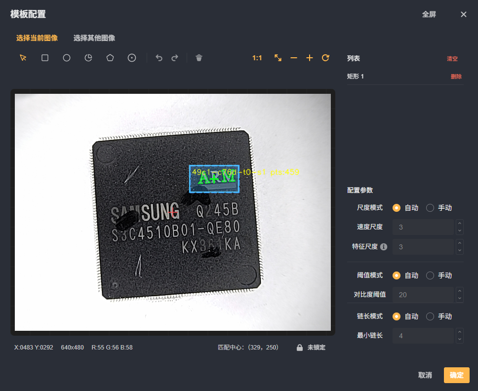
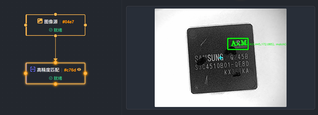
How It Works

The module first loads a pre-prepared template image, extracts key features such as its shape and edges, and generates a matching model. For the image to be inspected, the module slides a search window over the image according to the angle range and scale range set by the user, and calculates the similarity between the window content and the template features one by one. When the similarity reaches the set minimum match score, the position is recorded as a candidate target. Finally, all candidate targets are sorted by match score, and several targets with the highest score are output together with their sub-pixel accurate position, angle, and uniform or non-uniform scaling coefficients. By flexibly adjusting the angle step and the scale step, a balance between search efficiency and localization accuracy can be achieved.

Use Cases

High-precision localization of chips and pins in electronic component assembly, used to guide dispensing, soldering, or placement.
Position recognition before grasping mechanical parts, providing pick coordinates in scenarios with rotation or distance variation.
Alignment of labels and characters in the printing and packaging industry, ensuring cutting or lamination accuracy.
Multi-target finding and counting under complex background or occlusion conditions, such as automated sorting of pills, buttons, and similar items.

Parameters

Parameter	Description	Default Value
Search Mode	Whether to enable the "Search All" mode. When enabled, all possible targets in the entire image are searched; when disabled, other localization modules must be used to limit the search area.	Off
Minimum Match Score	Only targets whose match score is higher than this value are retained. The score range is 0~1 and two decimal places are supported. The higher the score, the more similar the target is to the template.	0.5
Maximum Number of Matches	Limits the maximum number of matching targets finally output, range 1~50000.	-
Matching Polarity	Polarity selection for template matching: 0 means normal polarity (the brightness relationship of the target is consistent with that of the template), 1 means inverted polarity (the brightness relationship of the target is opposite to that of the template).	-
Minimum Angle	The lower limit of the rotation angle search range, in degrees, value range -45~45.	-
Maximum Angle	The upper limit of the rotation angle search range, in degrees, value range -45~45.	-
Scale Range Type	Specifies how the scale range works: 0 means the X and Y directions use the same scale range, 1 means the X and Y directions can be set to different scale ranges independently.	0 (Uniform Scale)
Minimum Scale	When the scale range type is uniform scale, the minimum allowed scaling ratio, range 0.10~10.00.	1.00
Maximum Scale	When the scale range type is uniform scale, the maximum allowed scaling ratio, range 0.10~10.00.	1.00

Steps

Prepare the template: Use the template creation tool of Smart Vision Studio to select the target area from a typical image and generate a High-Precision Matching template, and save the template file to a user-specified directory.
Add the module: In the solution workflow, drag the "High-Precision Matching" module from the "Localization and Target Extraction" category to a suitable position, and connect the upstream image source or localization result to the input interface of the module.
Configure the template path: In the module parameter panel, select the pre-prepared template file through the "Browse" button.
Set the search parameters: According to the possible rotation and scaling range of the target to be inspected, configure the minimum/maximum angle, the scale range type, and the corresponding scaling parameters; adjust the minimum match score and the maximum number of matches according to the inspection requirements; if the polarity of the target is opposite to that of the background, check the matching polarity.
Run and verify: Execute a single step or a continuous run, observe the matching contours and scores drawn in the image area, and fine-tune the score threshold or the angle and scale ranges accordingly until all actually measured targets are stably detected.
Use the output results: Pass the coordinates, angle, and other information obtained from matching to subsequent measurement, recognition, or communication modules to complete localization guidance.

Contour Matching

Overview

The Contour Matching module is used to find targets in the input image that match a pre-learned contour template. By setting conditions such as the search angle range, the scale range, and the match score, localization can be completed when the target is rotated, scaled, or partially occluded. This module belongs to the "Matching" category of tools and is commonly used in scenarios such as workpiece localization and guided measurement that need to obtain the position and pose of a target.

How It Works

The Contour Matching module receives an image to be inspected and a contour template. During operation, the module searches for the template within the set region of interest according to the angle range and scale range specified by the user. At each candidate position, the module compares the similarity between the template contour and the edge features in the image and calculates a match score. When the match score reaches the set minimum match score and the number of matching targets does not exceed the maximum number of matches, the target is output as a valid result. The output usually includes information such as the position, angle, scale, and match score of the matching target. Parameters such as the search mode and the matching polarity affect the search strategy and the screening method.

Use Cases

Workpiece Localization: In scenarios such as robot grasping and assembly, identify the position and pose of parts with fixed shapes.
Defect Detection: By comparing with the standard contour, find missing, deformed, or extra parts of the target.
Classification and Recognition: When the target has differences in angle and scale, distinguish objects of different shapes.
Guided Measurement: Provide the approximate position and direction of the target for subsequent measurement tools to improve measurement efficiency.

Parameters

Parameter	Description	Default Value
Search Mode	Sets the search strategy for matching.
Minimum Match Score	The minimum score threshold for matching, value range 0~1, with two decimal places. Only targets whose match score is not lower than this value are output. Raising the threshold appropriately reduces false detections, and lowering it improves the detection rate.	0.5
Maximum Number of Matches	The maximum number of matching targets allowed to be output in a single inspection, value range 1~50000. Limiting the number of outputs avoids too many results.
Matching Polarity	Selects the matching polarity, used to specify the polarity condition for matching.
Minimum Angle	The minimum angle by which the template is allowed to rotate, value range -45~45 degrees. The lower limit of the angle by which the template can rotate during the search.
Maximum Angle	The maximum angle by which the template is allowed to rotate, value range -45~45 degrees. The upper limit of the angle by which the template can rotate during the search.
Scale Range Type	Selects the type of the scale range, used to control the way the scale changes.
Minimum Scale	The minimum allowed scale coefficient, value range 0.10~10.00. The lower limit of scale scaling during template matching.	1.00
Maximum Scale	The maximum allowed scale coefficient, value range 0.10~10.00. The upper limit of scale scaling during template matching.	1.00
Minimum Y Scale	Sets the minimum scale coefficient in the Y direction.
Maximum Y Scale	Sets the maximum scale coefficient in the Y direction.
Minimum X Scale	Sets the minimum scale coefficient in the X direction.
Maximum X Scale	Sets the maximum scale coefficient in the X direction.
Shape	Selects the shape type of the region of interest, including unspecified, rectangle, polygon, line caliper, circle caliper, and arc caliper. After selection, a detection area of the corresponding shape can be drawn on the image.
Start Point X	The X coordinate of the start point of the rectangle or caliper area.
Start Point Y	The Y coordinate of the start point of the rectangle or caliper area.
Width	The width of the rectangle area (unit: pixel).
Height	The height of the rectangle area (unit: pixel).
Rotation Angle	The rotation angle of the rectangle area (unit: degree).
Radius	The radius of the circle caliper or arc caliper (unit: pixel).
Circle Center X	The X coordinate of the circle center of the circle caliper.
Circle Center Y	The Y coordinate of the circle center of the circle caliper.
Number of Calipers	The number of calipers placed in the caliper detection area. The more calipers, the more detailed the inspection.
Caliper Width	The width of a single caliper (unit: pixel).
Caliper Height	The height of a single caliper (unit: pixel).
Arc Direction	The detection direction of the arc caliper, optional clockwise or counterclockwise.
Arc Size	The arc size type of the arc caliper, optional small arc or large arc.
Polygon Vertices	The list of vertex coordinates of the polygon area.

Steps

Add the "Contour Matching" module to the workflow of Smart Vision Studio.
Configure the template data path and select a pre-learned contour template.
Set parameters such as the minimum match score, the maximum number of matches, the angle range, and the scale range according to the actual inspection requirements.
Draw the region of interest on the image to limit the search range.
Run the module, view the matching results, and adjust the parameters as needed to optimize the detection effect.

Fast Matching

Fast Matching is a localization tool in the Matching category of Smart Vision Studio, used to quickly find the target area in an image that is most similar to a preset template. The module can adapt to changes in both the angle and the scale of the target, and, on the premise of ensuring the detection speed, returns one or more matching results that meet the similarity requirement.

When the inspection task has high requirements for cycle time and the target differs only in rotation, scaling, or brightness, the Fast Matching module is suitable for localization. It can help subsequent measurement, recognition, or alignment processes quickly lock onto the target position.

How It Works

The Fast Matching module receives an input image and template data and expands the search within the region of interest (ROI) set by the user. According to the set angle range and scale range, the module transforms the template at multiple angles and scales, and calculates the similarity between each candidate position in the image and the template one by one to obtain a match score.

All candidate positions are filtered according to the minimum match score, and only the results that reach the score threshold are retained. The module then sorts the results by match score and limits the final number of output targets according to the maximum number of matches. The output results usually include the position of the target in the image, the rotation angle relative to the template, the scaling ratio, and the match score.

By limiting the search area, the angle range, the scale range, and the number of matches, Fast Matching can significantly shorten the processing time while maintaining high stability, making it suitable for online localization applications.

Parameters

Parameter	Description	Default Value
Search Mode	Switches whether to use the search all mode. When enabled, all matching targets that meet the conditions are searched within the entire search range.
Minimum Match Score	The similarity threshold of the matching result, value range 0~1, with two decimal places. Only candidate positions that reach this score are retained. The higher the score, the more reliable the result, but some targets may be missed; the lower the score, the looser the matching, but false detections may be introduced.	0.5
Maximum Number of Matches	The maximum number of matching targets returned, value range 1~50000. It is recommended to set it according to actual needs to avoid returning too many invalid results.
Matching Polarity	Controls the polarity handling method during matching. The value is 0 or 1, corresponding to different polarity strategies. For the specific meaning, refer to the interface option prompt.
Minimum Angle	The minimum rotation angle allowed during the search, range -45°~45°. Usually set to the lower limit of the possible rotation range of the target.
Maximum Angle	The maximum rotation angle allowed during the search, range -45°~45°. Usually set to the upper limit of the possible rotation range of the target.
Scale Range Type	Selects the control method of the scale range. You can set the overall scale uniformly, or set the scale ranges of the X and Y directions separately. When non-uniform scaling is required, select the separate setting mode.
Minimum Scale	The minimum scaling ratio of the matching target relative to the template, range 0.10~10.00.	1.00
Maximum Scale	The maximum scaling ratio of the matching target relative to the template, range 0.10~10.00.	1.00
Minimum Y Scale	When the scale range type is separate setting, the minimum scaling ratio in the Y direction.
Maximum Y Scale	When the scale range type is separate setting, the maximum scaling ratio in the Y direction.
Minimum X Scale	When the scale range type is separate setting, the minimum scaling ratio in the X direction.
Maximum X Scale	When the scale range type is separate setting, the maximum scaling ratio in the X direction.
Shape	Selects the shape type of the region of interest. The optional shapes include unspecified, rectangle, polygon, line caliper, circle caliper, arc caliper, and so on. The specific available shapes are subject to the interface display.	Unspecified
Start Point X	The X coordinate of the start point of the rectangle or caliper area.
Start Point Y	The Y coordinate of the start point of the rectangle or caliper area.
Width	The width of the rectangle area, in pixels.
Height	The height of the rectangle area, in pixels.
Rotation Angle	The rotation angle of the rectangle area, in degrees.
Radius	The radius of the circle caliper or arc caliper, in pixels.
Circle Center X	The X coordinate of the circle center of the circle caliper.
Circle Center Y	The Y coordinate of the circle center of the circle caliper.
Number of Calipers	The number of calipers placed in the caliper detection area. The more calipers, the more detailed the inspection.
Caliper Width	The width of a single caliper, in pixels.
Caliper Height	The height of a single caliper, in pixels.
Arc Direction	The detection direction of the arc caliper, optional clockwise or counterclockwise.
Arc Size	The arc size type of the arc caliper, optional small arc or large arc.
Polygon Vertices	The list of vertex coordinates of the polygon area.

Steps

Add the "Fast Matching" module to the workflow.
Connect the input image and the template data, and make sure the template has been generated or imported correctly.
Set the region of interest (ROI) as needed, draw the detection range, and exclude irrelevant areas.
Configure the matching parameters, including the minimum match score, the maximum number of matches, the angle range, and the scale range.
If the target is scaled non-uniformly in the X and Y directions, switch the scale range type to separate setting, and adjust the scale ranges in the X and Y directions separately.
Run the flow and check the matching position, angle, scaling ratio, and match score output by the module.
Fine-tune the parameters according to the actual results until the inspection requirements are met.

Grayscale Matching

Grayscale Matching is an inspection module in Smart Vision Studio used to locate a target object in an image. Taking a pre-created template as the reference, the module searches the specified area of the input image for the target that is most similar to the grayscale features of the template, and returns information such as the position, angle, scale, and match score of the target.

When an inspection task needs to determine the specific position and pose of a target in an image and the appearance of the target is mainly characterized by grayscale texture, the Grayscale Matching module can be selected. It can effectively handle situations where the target has a certain degree of rotation, scale change, or partial occlusion, and provides reliable reference information for subsequent tasks such as measurement, recognition, or localization guidance.

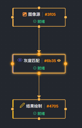
How It Works

When the Grayscale Matching module runs, it first obtains the pre-created template data, which records the grayscale features of the target object. The module then traverses the region of interest of the input image according to the set search mode, and calculates the grayscale similarity between each candidate position in the image and the template to obtain the corresponding match score.

During the search, the module rotates and scales the template according to the angle range and scale range set by the user, so as to match targets with different poses that may exist in the image. Finally, the module screens out the results that meet the minimum score requirement in descending order of match score, and returns the position coordinates, angle, scale, and match score of each matching result.

Parameters

Parameter	Description	Default Value
Search Mode	Selects whether to use the search all mode during matching. When enabled, the search space is traversed more thoroughly, which improves the probability of finding the target, but increases the computation time.	Off
Minimum Match Score	The minimum score threshold for determining a valid matching result, with a value range of 0 to 1 and two decimal places. The higher the score, the stricter the similarity requirement for matching and the lower the false detection rate, but some targets may be missed.	0.5
Maximum Number of Matches	The maximum number of targets allowed to be returned in a single inspection, with a value range of 1 to 50000. It can be set according to the maximum number of targets that may appear in the field of view.	To be confirmed
Matching Polarity	Specifies the grayscale contrast direction between the template and the image. Different polarity options correspond to different grayscale matching methods, and the selection must be based on the actual grayscale relationship between the target and the background.	To be confirmed
Minimum Angle	The minimum rotation angle allowed for the search, with a value range of -45° to 45°. Together with the maximum angle, it forms the angle search range.	To be confirmed
Maximum Angle	The maximum rotation angle allowed for the search, with a value range of -45° to 45°. The wider the angle range is set, the more poses can be matched, but the longer the processing time.	To be confirmed
Scale Range Type	Selects the way the scale range is set. Different options correspond to uniform scale (proportional scaling in the X and Y directions) or per-axis scale (the scaling ranges in the X and Y directions are set separately).	To be confirmed
Minimum Scale	The minimum scaling ratio allowed for matching in uniform scale mode, with a value range of 0.10 to 10.00.	1.00
Maximum Scale	The maximum scaling ratio allowed for matching in uniform scale mode, with a value range of 0.10 to 10.00.	1.00
Minimum Y Scale	The minimum scaling ratio allowed for matching in the Y direction in per-axis scale mode.	To be confirmed
Maximum Y Scale	The maximum scaling ratio allowed for matching in the Y direction in per-axis scale mode.	To be confirmed
Minimum X Scale	The minimum scaling ratio allowed for matching in the X direction in per-axis scale mode.	To be confirmed
Maximum X Scale	The maximum scaling ratio allowed for matching in the X direction in per-axis scale mode.	To be confirmed
Shape	Selects the shape type of the region of interest. The options are unspecified, rectangle, polygon, line caliper, circle caliper, or arc caliper.	Unspecified
Start Point X	The X coordinate of the start point of the rectangle or caliper area.	To be confirmed
Start Point Y	The Y coordinate of the start point of the rectangle or caliper area.	To be confirmed
Width	The width of the rectangle area (unit: pixel).	To be confirmed
Height	The height of the rectangle area (unit: pixel).	To be confirmed
Rotation Angle	The rotation angle of the rectangle area (unit: degree).	To be confirmed
Radius	The radius of the circle caliper or arc caliper (unit: pixel).	To be confirmed
Circle Center X	The X coordinate of the circle center of the circle caliper.	To be confirmed
Circle Center Y	The Y coordinate of the circle center of the circle caliper.	To be confirmed
Number of Calipers	The number of calipers placed in the caliper detection area. The more calipers, the more detailed the inspection.	To be confirmed
Caliper Width	The width of a single caliper (unit: pixel).	To be confirmed
Caliper Height	The height of a single caliper (unit: pixel).	To be confirmed
Arc Direction	The detection direction of the arc caliper, optional clockwise or counterclockwise.	To be confirmed
Arc Size	The arc size type of the arc caliper, optional small arc or large arc.	To be confirmed
Polygon Vertices	The list of vertex coordinates of the polygon area.	To be confirmed

Steps

In the workflow editing area of Smart Vision Studio, add the Grayscale Matching module from the Matching category.
Connect the output of the image to be inspected to the input port of the Grayscale Matching module, and make sure the image data can be passed in normally.
Connect the pre-created template data to the template input port of the module.
In the parameter interface, set an appropriate region of interest according to the possible position of the target in the image. Usually the region of interest is limited to the range in which the target may appear, so as to reduce the search time and exclude interference outside the area.
Set the angle range and the scale range according to the pose changes of the target. If the target may be rotated, relax the angle range appropriately; if the size of the target may change, set the corresponding scale range.
Set the minimum match score and the maximum number of matches. The match score threshold can be adjusted according to the actual similarity between the template and the target. Usually the default value is kept during the initial test, and then optimized step by step according to false detections or missed detections.
Run the flow and observe the matching results that are output. If the matching effect is not satisfactory, adjust parameters such as the region of interest, the angle range, or the match score until a stable localization effect is obtained.

Measurement

Point-to-Point Measurement

Point-to-point measurement is used to calculate the geometric relationship between any two points in an image, including the straight-line distance and the direction angle. This module is usually used in situations where the spacing or the relative direction of two feature positions needs to be obtained, such as the measurement of the spacing between locating holes or the calculation of the included angle of a workpiece edge. After the user specifies the image coordinates of the start point and the end point, the module can quickly give accurate measurement results and pass the results to the downstream flow for continued use.

The point-to-point measurement module is generally used together with localization modules such as circle finding. Modules such as circle finding act as the preceding module

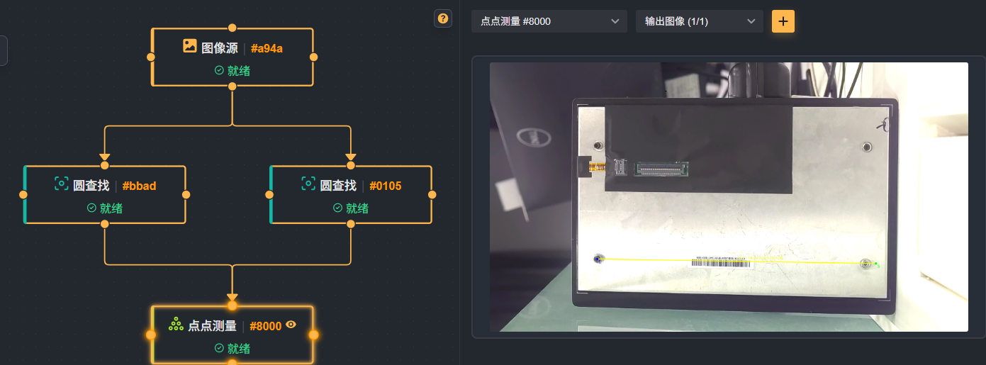
How It Works

The module receives the coordinates of two points (the start point and the end point) and calculates the Euclidean distance between them and the direction angle of the connecting line in the selected coordinate system. The distance is given in pixels; the direction angle is output according to the set angle range, which can be -90° to 90° or -180° to 180°. The coordinate system defaults to the image coordinate system, that is, a rectangular coordinate system with the upper-left corner of the image as the origin, the X axis pointing to the right, and the Y axis pointing downward. The calculation process is entirely based on geometric formulas and does not involve the image content itself, so it runs fast and is suitable for any scenario in which the point positions have been determined.

Use Cases

Detect the actual distance between the centers of two circular holes and determine whether it meets the assembly tolerance.
Calculate the inclination angle of the line connecting two points on a workpiece edge, used for localization rotation compensation.
Together with other localization tools, measure the offset between the template matching result and the reference point.
In a calibrated image, obtain the pixel distance before converting it into a physical dimension.

Parameters

Parameter	Description	Default Value
Start Point X	The X-axis pixel coordinate of the start point. The origin of the coordinate system is at the upper-left corner of the image, and the X axis is horizontal to the right.
Start Point Y	The Y-axis pixel coordinate of the start point. The Y axis is vertical downward.
End Point X	The X-axis pixel coordinate of the end point.
End Point Y	The Y-axis pixel coordinate of the end point.
Coordinate System	Selects the coordinate system type. 0 is the image coordinate system; for other possible values, refer to the prompts in the product interface.	0
Angle Range	The representation range of the output angle. 0: -90° to 90°; 1: -180° to 180°. It affects the sign and the value interval of the angle.	1

This module is based on pure coordinate calculation and does not directly process the image content. Therefore, make sure that the input coordinates have been obtained in a reliable way, and avoid passing in irrelevant or wrong points.
The choice of the angle range changes the sign and the value of the output angle. After the range is switched, the angle value may change, so keep it consistent with the subsequent judgment logic.
If the image coordinate system is used, the Y axis points downward, and the angle calculation follows the right-hand rule. Users need to pay attention to the correspondence with the actual spatial direction.
The distance output by the module is a pixel distance. To obtain a physical unit such as millimeters, convert it with the calibration module.

Point-to-Line Measurement

The point-to-line measurement module is used to calculate the perpendicular distance from a given point to a specified line, the coordinates of the foot of the perpendicular, and the relative included angle between the point and the line. In quality inspection, it is often necessary to evaluate the deviation of a point feature (such as a hole center or a corner point) relative to a reference edge or a reference line. This module directly provides accurate geometric values to help users quickly make a pass/fail judgment.

The point-to-line measurement module is generally used together with localization modules such as circle finding and line finding. Modules such as circle finding and line finding act as the preceding module

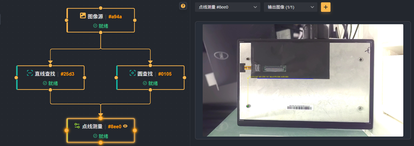
How It Works

The module receives the point coordinates entered by the user and the coordinates of a line defined by a start point and an end point. According to the selected coordinate system, the positions of the point and the line are unified into the same reference frame, and geometric methods are then used to calculate the perpendicular distance from the point to the line (signed, indicating which side of the line the point is on), the coordinates of the foot of the perpendicular, and the angle formed by the point and the line. The angle output range can be selected by the user to suit different direction judgment requirements. Finally, the module outputs the measurement results for use by the subsequent flow or for direct display.

Use Cases

Detect whether the perpendicular distance from the center of a locating hole to the product edge is within the tolerance range.
Measure the collinearity of multiple points, and evaluate straightness by comparing the deviation of each point from the same reference line.
Check the alignment of the corner point of a workpiece with the reference line, commonly used for assembly position deviation analysis.
Together with other modules (such as circle finding and edge extraction), implement automated geometric dimension measurement.

Parameters

Parameter	Description	Default Value
Point X Coordinate	The X coordinate of the point to be measured. A numeric value can be entered manually, or the output variable of another module can be bound.	None
Point Y Coordinate	The Y coordinate of the point to be measured, bound in the same way as above.	None
Line Start Point X	The X coordinate of the start point of the reference line. When used together with modules such as edge fitting, it can be obtained through a variable.	None
Line Start Point Y	The Y coordinate of the start point.	None
Line End Point X	The X coordinate of the end point of the reference line. The two points together determine a unique line.	None
Line End Point Y	The Y coordinate of the end point.	None
Coordinate System	Selects the coordinate system on which the input coordinates are based. Currently the image coordinate system is supported (the origin is at the upper-left corner of the image).	Image Coordinate System
Angle Range	Sets the representation range of the output angle: -90°~90° outputs an acute angle, reflecting only the degree of inclination; -180°~180° can express the complete circular direction and makes it easier to distinguish the orientation.	-180°~180°

The coordinates of the point and the line must belong to the same coordinate system; otherwise the calculation result is invalid.
The start point and the end point of the line must not coincide; otherwise the line cannot be uniquely determined and the module returns an error state.
The sign of the perpendicular distance can be used to determine whether the point is on the left or the right side of the line. Verify the sign definition in actual tests to avoid misjudging the direction.
The setting of the angle range affects the output value domain, so make sure it matches the subsequent logic. For example, when the angle is used as a rotation angle, select -180°~180°.
When the input coordinates come from an upstream module, pay attention to the module execution order and make sure the relevant data has been generated and is valid before the point-to-line measurement.

Line-to-Line Measurement

The line-to-line measurement module is used to accurately calculate the geometric relationship between two lines. Typical applications include angle measurement, parallelism determination, and spacing calculation. In scenarios such as localization, guidance, and inspection, the user can specify the end points of two lines on the image, and the module automatically extracts the edges and fits the lines, and finally outputs key parameters such as the included angle of the two lines or the distance between them.

The line-to-line measurement module is generally used together with localization modules such as line finding. Modules such as line finding act as the preceding module

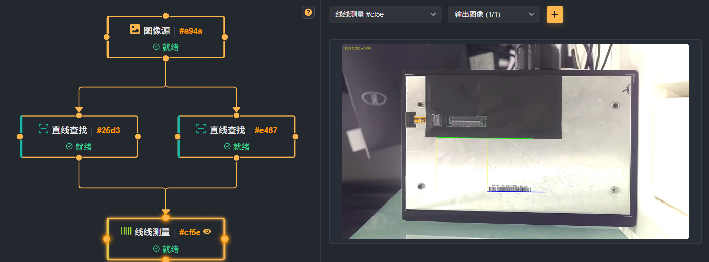
How It Works

The module first receives the end point coordinates of the two lines and creates several rectangular sampling areas in the direction of the line connecting the end points of each line. In each sampling area, edge points are found according to the set edge polarity, edge threshold, and filter size, and abnormal edge points are removed according to the rejection distance and the number of rejected points. Then, the retained edge points are fitted into a line using the specified initial fitting strategy and fitting method. Finally, according to the selected line and the set angle range, the angle or the distance between the two lines is calculated and output.

This flow combines edge extraction with line fitting, which can effectively suppress image noise and local interference, and provides stable and reliable results for tasks such as angle measurement and parallelism detection.

Use Cases

Workpiece Angle Measurement: Detect whether the included angle of a part edge meets the design requirements, such as the bending angle of sheet metal.
Parallelism/Perpendicularity Detection: Verify whether two edges are parallel or perpendicular after the product is assembled, such as the alignment of the battery electrode sheet and the separator.
Distance Measurement: Calculate the spacing between two approximately parallel edges, such as the gap width or the slot width.
Guidance and Alignment: Provide the included angle information of the two lines for a robot arm or a mounting head to implement rotation compensation.

Parameters

Parameter	Description	Default Value
Coordinate System	Specifies the coordinate system of the measurement reference. The image coordinate system is supported.	Image Coordinate System
Output Angle Range	Defines the representation interval of the output angle: -90°~90° or -180°~180°. Different intervals suit workpieces placed at different angles and prevent the angle output from jumping.	-180°~180°
Select Line	Specifies the target line whose angle or distance is to be measured. Select "Line 1" or "Line 2", and the module outputs the included angle between that line and the other line; later versions may also use it for distance output.	-
Edge Type	Determines the edge point search strategy: the strongest edge, the last edge, the first edge, or the edge near the center line. Different modes affect the order in which the finally fitted line responds to image features.	Strongest
Edge Polarity	Defines the edge transition mode: any polarity, black to white, or white to black. Select it according to the contrast direction of the target edge to exclude interference from reverse edges.	Any Polarity
Edge Threshold	The sensitivity of edge detection, with a value range of 1-255. The smaller the value, the more weak edges are included as candidate points; the larger the value, the more only edges with strong contrast are retained.	5
Filter Size	The window size for smoothing filtering before edge detection, with a value range of 1-50. A larger value can suppress noise, but it reduces edge localization accuracy.	1
Number of Rejected Points	The number of outliers removed from the set of edge points before fitting the line, with a value range of 0-998. Together with the rejection distance, it removes obvious wrong edge points.	0
Rejection Distance	Defines the distance threshold for judging outliers, with a value range of 1-1000 pixels. Points whose distance from the fitted line exceeds this value are regarded as outliers (within the limit of the number of rejected points).	5
Initial Fitting	Selects the initial fitting strategy: global or local. Global fitting uses all sampling points to fit at one time and is fast; local fitting fits in segments and then combines them, which adapts better to local deformation.	Local
Fitting Method	The mathematical method of line fitting: least squares, Huber, or Tukey. Least squares is optimal for normally distributed errors; Huber and Tukey are more robust against abnormal points.	Huber

The Edge Threshold and Polarity Must Match the Actual Contrast: If the contrast of the target edge in the image is low, lower the edge threshold appropriately, and make sure the polarity is set correctly; otherwise edges may be missed or reverse edges may be introduced.
The Rejection Parameters Should Not Be Too Large: Too many rejected points or too small a rejection distance may reject valid edge points, leading to inaccurate line fitting. Observe the distribution of the edge points first and then adjust step by step.
The Filter Size Affects Localization Accuracy: On the premise of ensuring the denoising effect, use a filter size as small as possible to avoid a shift in the edge position.
Selection of the Angle Range: If the placement angle of the workpiece being measured may exceed 90°, use the -180°~180° interval to prevent the angle output from jumping.
Matching Between the Fitting Method and the Initial Fitting: When very few large outliers exist on the edge, prefer Tukey fitting; if the edge is relatively regular, using least squares improves the calculation speed.

Line-to-Circle Measurement

The line-to-circle measurement module is used to calculate the geometric relationship between a line and a circle. When an inspection task needs to obtain the shortest distance from an edge point to the circle center, or to evaluate the position deviation of a circular workpiece relative to a line reference, this module can be selected. It outputs key measurement data such as the distance from the line to the circle and the intersection point coordinates, helping users quickly determine whether a workpiece meets the tolerance requirements.

The line-to-circle measurement module is generally used together with localization modules such as line finding and circle finding. Modules such as line finding and circle finding act as the preceding module

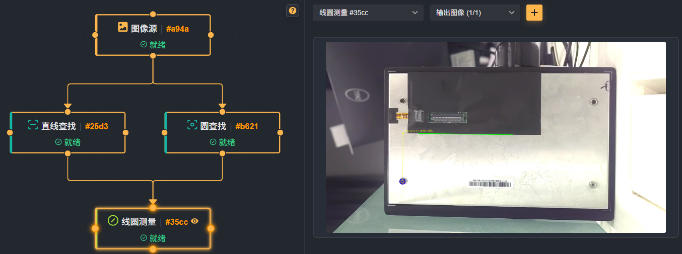
How It Works

The module receives a line and a circle as the input reference. The line is defined by a start point and an end point, and the circle is defined by the center coordinates and the radius. The module first determines the calculation direction according to the selected coordinate system and angle range, and then solves the geometric relationship between the line and the circle. Finally, it outputs complete results such as the distance from the line to the circle center, the coordinates of the foot of the perpendicular, the line-circle intersection points, and the projection point of the circle center on the line. The whole calculation process is based on analytical geometry methods and can stably handle various positional relationships such as separation, tangency, and intersection.

Use Cases

Distance Measurement from a Workpiece Edge to a Hole Position: Using the line fitted to the workpiece edge as the reference, measure the distance from the center of a circular hole to the edge.
Pin Position Detection: Using the product boundary line as the reference, detect the offset of a circular pin or locating post relative to the boundary.
Angle Evaluation Between a Circular Feature and the Reference Line: Analyze the degree of deviation between the center of a circular feature and the ideal reference line.
Tangent Point Position Verification: When a circle is required to be tangent to a certain line, verify whether the actual tangent point coordinates meet the design requirements.

Parameters

Parameter	Description	Default Value
Line Start Point X/Y	Defines the abscissa and the ordinate of the start point of the input line respectively. This point is usually subscribed from an upstream module, or a fixed value can be entered manually.	None
Line End Point X/Y	Defines the abscissa and the ordinate of the end point of the input line respectively. The start point and the end point together determine the direction of the line and the calculation reference.	None
Circle Center X/Y	Defines the center position of the input circle. The coordinate values must match the current coordinate system.	None
Measurement Radius	The radius value of the input circle. Together with the circle center position, it determines the boundary of the circle and directly affects the accuracy of the intersection point calculation.	None
Coordinate System	Specifies the coordinate system on which the calculation is based. In the image coordinate system, the X axis is positive to the right and the Y axis is positive downward.	Image Coordinate System
Output Angle Range	Sets the value range of the output angle. Selecting -90° to 90° is suitable for most measurements that are mainly in the horizontal direction; selecting -180° to 180° provides complete angle information and is suitable for full-circumference evaluation.	-180°~180°
Selection Type	Specifies the reference feature used in the current measurement. A line or a circle can be selected as the reference for the distance and angle calculation.	Line 1

Drag the "Line-to-Circle Measurement" module from the toolbox to the workflow editing area.
Subscribe upstream data sources for the "Line" and "Circle" inputs respectively, for example the output line of the line finding module and the output circle of the circle finding module.
If the positioning reference in the image coordinate system has not been subscribed, confirm that the "Coordinate System" parameter is the image coordinate system. If necessary, switch to the physical coordinate system after pixel-level calibration.
Set an appropriate "Output Angle Range" according to the actual inspection requirements.
Run the flow and view the output data such as the distance, the coordinates of the foot of the perpendicular, and the intersection points in the result display area.
Together with the subsequent judgment or output modules, complete the dimension tolerance judgment or the data export.

Circle-to-Circle Measurement

The circle-to-circle measurement module is used to accurately calculate the geometric relationship between two circles. The most typical application is to obtain the distance between the centers of the two circles and the angle of the line connecting the centers. When an inspection task needs to measure the hole spacing, the coaxiality, or the assembly position deviation, this module can quickly extract the required dimension information from the two circles that have already been located, without manual calculation. The module supports selecting the representation range of the output angle to suit different angle measurement habits.

The circle-to-circle measurement module is generally used together with localization modules such as circle finding. Modules such as circle finding act as the preceding module

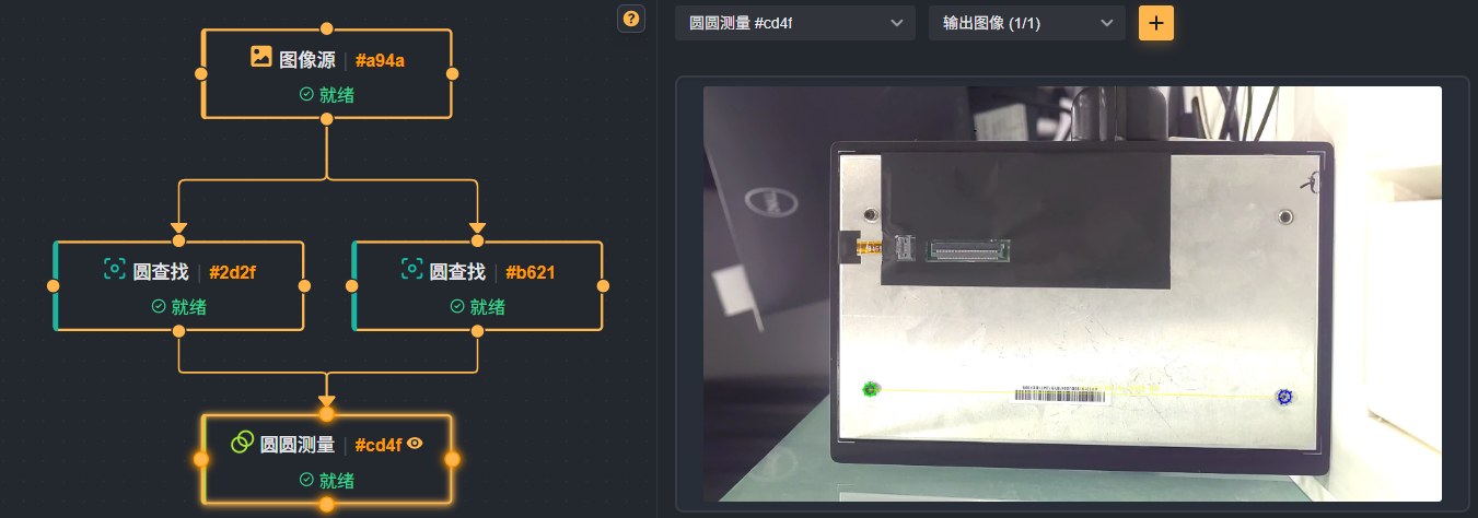
How It Works

The module receives the basic parameters of two circles from the previous process, including the center coordinates and the radius of each circle. Internally, the module first establishes the calculation reference according to the coordinate system and angle range configuration selected by the user. Then, it calculates the Euclidean distance between the two circle centers and the direction angle of the line connecting the centers from the two preset circle parameters. The output range of the angle value can be normalized between -90°~90° or -180°~180° as set by the user, so that it can be directly used for dimension judgment or transmitted to a subsequent tolerance judgment module. The whole process does not need to fit the circles again, but directly uses the existing circle data to complete the measurement, which reduces repeated calculation and improves the flow efficiency.

Use Cases

Hole spacing measurement: Detect whether the center distance of two circular holes on a workpiece is within the tolerance range.
Assembly deviation detection: Determine whether the relative position of two circles (such as a bearing seat and a shaft hole) meets the assembly requirements.
Angle alignment verification: Measure the angle of the line connecting the centers of the two circles relative to the horizontal axis, used for direction positioning inspection.
Preliminary coaxiality evaluation: Quickly screen for coaxiality abnormalities by analyzing the inclination angle of the line connecting the two circle centers.

Parameters

Parameter	Description	Default Value
Coordinate System Selection	Selects the coordinate system used as the reference for the calculation. The image coordinate system is usually used, in which the origin is located at the top-left corner of the image, the X axis points to the right, and the Y axis points downward.	Image Coordinate System
Output Angle Range	Sets the representation range of the direction angle of the line connecting the two circle centers. The options are -90°~90° or -180°~180°. The former limits the angle to the right half-plane, while the latter allows the full circular angle to be output.	-180°~180°

Add the circle-to-circle measurement module to the workflow and place it after the two circle finding modules.
Connect the two circle parameters output by the preceding modules to the corresponding input ports of this module.
In the module parameter area, select the appropriate "Coordinate System Selection" option.
Adjust the "Output Angle Range" option according to the angle range required by the subsequent judgment.
Run the workflow. The circle center distance, the angle of the line connecting the circle centers, and the current parameters of the two circles can then be viewed in the result display area.

Point-to-Circle Measurement

The point-to-circle measurement module is used to calculate and output the relative position information between a point and a circle in an image. When the distance or the azimuth from a certain point to a specified circle center needs to be determined, you can use this module. Typical applications include checking whether a feature point falls within a circular region and evaluating the angular deviation of a point relative to a reference circle. It is a basic geometric relationship judgment tool in the Measurement category.

The point-to-circle measurement module is generally used together with localization modules such as circle finding. Modules such as circle finding act as the preceding module

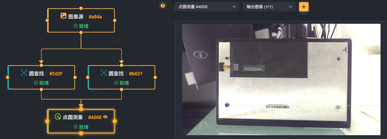
How It Works

According to the point coordinates and circle parameters provided by the user (circle center coordinates and radius), the module calculates the distance between the point and the circle center in the selected coordinate system, and at the same time calculates the angle of the line connecting the point and the circle center relative to the horizontal direction. The output range of the angle can be adjusted through parameters to suit different conventions of direction expression (for example, -90°~90° or -180°~180°). All calculation results are output as standard measurement fields for use by downstream modules or for the display of the final result. Since the calculation depends only on the given coordinates and parameters, the module does not need to rely on the image or on preceding localization tools and can participate in the measurement flow independently.

Use Cases

Check whether a certain feature point is located within a circular datum region, for example, to judge whether a solder joint deviates from the circular tolerance zone.
Measure the angle from the center of a locating hole on a part to a corner point to assist pose calculation.
In text or pattern inspection, judge the angular offset of the pattern center relative to a reference circle.
Together with other measurement modules, use the relationship between the point and the circle as a feature value for dimension judgment.

Parameters

Parameter	Description	Default Value
Point X Coordinate	The horizontal coordinate of the point to be measured. This value usually comes from the point coordinates output by an upstream module, and can also be entered manually.	-
Point Y Coordinate	The vertical coordinate of the point to be measured.	-
Circle Center X Coordinate	The horizontal coordinate of the center of the reference circle.	-
Circle Center Y Coordinate	The vertical coordinate of the center of the reference circle.	-
Circle Radius	The radius of the reference circle, used to determine the position and size of the circle.	-
Coordinate System	Defines the reference frame on which the coordinate calculation is based. When "Image Coordinate System" is selected, the coordinate origin is located at the top-left corner of the image, the positive X direction points to the right, and the positive Y direction points downward.	Image Coordinate System
Angle Range	Controls the range of the output angle. 0 means the output angle is between -90° and 90°; 1 means the output angle is between -180° and 180°. You can choose according to the actual convention of angle expression.	1 (-180°~180°)

In the measurement tool group of Smart Vision Studio, find the "Point-to-Circle Measurement" module and add it to the workflow editing area.
Click the module, and in the parameter configuration area enter the coordinates of the measurement point and the circle center coordinates and radius of the reference circle. These values can be filled in directly, or obtained dynamically by binding the output variables of other modules.
Select the coordinate system type according to actual needs (usually keep the default "Image Coordinate System").
Set the angle range. If you need to distinguish the clockwise/counterclockwise direction or the full circular angle, select the -180°~180° range; if you only care about acute angles or angle values in a smaller interval, select the -90°~90° range.
Run the flow and view the output distance and angle information in the result display area. The module also passes all output values to subsequent modules for further calculation or judgment.

Calibration and Coordinates

Calibration Board Calibration

Calibration board calibration is used to establish the correspondence between image pixel coordinates and actual physical coordinates, and is a basic step in applications such as visual measurement, localization, and robot guidance. When the position and distance recognized in the image need to be converted into an actual spatial position or physical length, use this module to complete the calibration.

This module detects the calibration board features in the image and, together with parameters such as the calibration board description file and the physical size, calculates the transformation relationship between pixel coordinates and physical coordinates. The calibration result can be called directly by subsequent modules such as measurement and localization modules, thereby ensuring the accuracy and consistency of the output of the vision system.

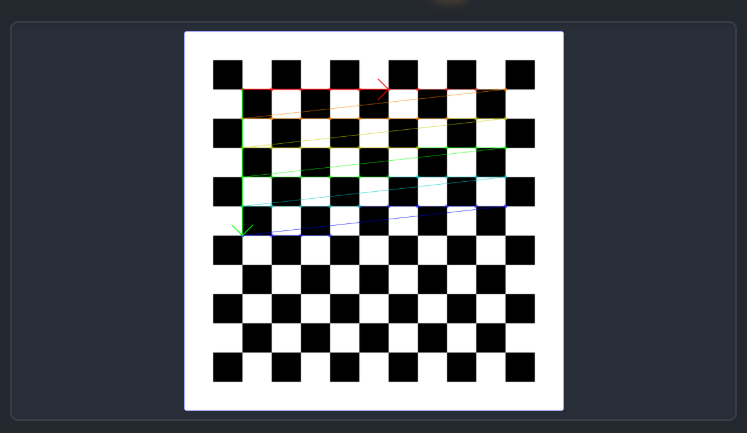
Use Cases

Perform the first calibration after the camera is installed, to eliminate the coordinate deviation caused by the lens installation angle and the imaging position.
In high-precision dimension measurement, convert the pixel distance in the image into an actual physical distance such as millimeters or micrometers.
In robot visual localization and picking, convert the coordinates of the workpiece recognized by vision into the robot coordinate system.
When the imaging system has tilt or perspective distortion, perform coordinate correction to improve the overall localization precision.

Parameters

Parameter	Description	Default Value
Calibration Board File	Specifies the calibration board description file. Through this file, the module obtains necessary information such as the layout and type of the calibration board pattern. Only when the file path is valid and matches the actual calibration board can feature recognition and calibration be completed correctly.	No default value; the user must specify it
Calibration Board Type	Selects the type of calibration board pattern actually used. The current version supports the chessboard calibration board. Selecting a wrong type causes feature detection to fail or reduces the calibration precision.	Chessboard Calibration Board
Physical Size	Defines the actual physical size corresponding to the calibration board pattern; it is the basis for converting pixel distances into actual physical lengths. This value directly affects the final measurement scale, so it must be filled in according to the actual calibration board and the unit must be kept consistent. Value range: 0.01 ~ 1000.00.	1.00
Coordinate System Mode	Determines whether the calibration result uses a left-handed or a right-handed coordinate system. This setting must be consistent with the coordinate system used by subsequent localization modules or by the robot or worktable; otherwise the coordinate direction may be mirrored or reversed.	Left-Handed Coordinate System
Origin (X)	Sets the offset of the calibration board coordinate system origin in the X direction. The default origin is 0, which means the default position of the calibration board pattern is used as the origin; if the coordinate origin needs to be translated to a specific position, adjust this value. Value range: -1000.00 ~ 1000.00.	0
Origin (Y)	Sets the offset of the calibration board coordinate system origin in the Y direction. The default origin is 0, which means the default position of the calibration board pattern is used as the origin; if the coordinate origin needs to be translated to a specific position, adjust this value. Value range: -1000.00 ~ 1000.00.	0
Rotation Angle	Defines the rotation angle of the calibration board coordinate system relative to the reference direction, in degrees. When the installation direction of the calibration board is not consistent with the target coordinate axis, this angle can be used for correction. Value range: -180.00 ~ 180.00.	0
Degrees of Freedom	Controls the complexity of the calibration transformation model. The options include: scale, rotation, translation; scale, rotation, aspect ratio, tilt, translation; and scale, rotation, aspect ratio, tilt, translation, and perspective. The higher the degrees of freedom, the more complex the geometric deformation that can be corrected, but the higher the requirement for the quality of the feature points.	Scale, Rotation, Aspect Ratio, Tilt, Translation, and Perspective
Median Filter Status	Sets whether median filtering is performed on the image before calibration. Filtering is performed by default, which can effectively reduce the interference of noise with feature detection. If the image is clear with little noise and processing speed is required, filtering can be turned off.	Perform Filtering

Notes

Before calibration, make sure the calibration board appears completely in the image with all features clearly visible, and avoid strong reflection, occlusion, or overexposure.
The physical size must be completely consistent with the actual calibration board, and the unit must be kept consistent; an incorrect entry causes a proportional deviation in the measurement result.
The coordinate system mode and the rotation angle must be consistent with the coordinate system used later, to avoid deviation in the coordinate direction or the origin position.
The degrees of freedom are not the higher the better; choose them according to the actual imaging distortion. Unnecessary degrees of freedom reduce the stability of the calibration result.
Median filtering is enabled by default and suits most scenarios. If the image details are already relatively smooth or you are sensitive to processing speed, you can turn filtering off.

Unit Conversion

The unit conversion module is used in the calibration and coordinate processing flow to convert the pixel distance in an image into an actual physical size. When the measurement or localization result needs to be output in engineering units such as millimeters or micrometers, you can use this module to complete the conversion from pixels to physical units. It also supports fine-tuning an existing calibration relationship to adapt to on-site environmental changes or mechanical installation errors.

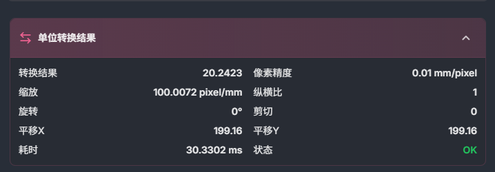
How It Works

The module receives a calibration file and the pixel distance to be converted. The calibration file records the correspondence between pixels and physical sizes under the current camera imaging conditions. The module converts the input pixel distance according to this relationship and outputs the physical distance. If a pixel scale correction is set, the module adjusts the original conversion relationship proportionally so that the result is closer to the actual size. The refresh signal is used to trigger recalculation after the calibration file or the input data is updated, ensuring that the output is consistent with the latest configuration.

Use Cases

In visual measurement, the detected pixel length needs to be converted into millimeters or micrometers.
After the camera is recalibrated, the coordinate units of different stations or devices need to be unified.
Perform local correction of an existing calibration relationship to compensate for errors caused by installation or environmental changes.
Convert the pixel coordinates output by the preceding localization module into physical coordinates for subsequent control or statistics.

Parameters

Parameter	Description	Default Value
Calibration File	Specifies the location of the calibration file used for unit conversion. This file is usually generated by the camera calibration flow and contains the correspondence between pixels and actual physical sizes. An incorrect path or an invalid file causes the conversion to fail or the result to deviate.	No default value
Pixel Scale Correction	Proportionally adjusts the current calibration relationship to correct deviations caused by environmental changes, mechanical installation errors, and so on. Increasing this value makes the physical distance corresponding to the same pixel distance larger.	No default value
Pixel Distance	The pixel distance to be converted, usually coming from the output of a preceding measurement or localization module.	No default value
Refresh Signal	The control signal that triggers the module to perform the conversion again. When the calibration file, the pixel distance, or the correction value changes, this signal makes the module update the result.	No default value

Notes

Make sure the calibration file path is correct and the file is accessible; otherwise the module cannot complete the conversion.
Pixel scale correction proportionally affects all conversion results; when adjusting it, verify with a standard part of known size.
The input pixel distance must be consistent with the camera and imaging conditions corresponding to the calibration file; recalibration is required for a different camera or a different working distance.
If the refresh signal is not triggered, the module may keep the last calculation result; after the data is updated, confirm that the signal is configured correctly.
Changes to the calibration file change the conversion baseline. After replacing the calibration file, re-check whether the conversion results are reasonable.

Recognition and Code Reading

Code Reading

The code reading module is used to recognize and read the encoded content of code symbols from the input image and belongs to the "Recognition and Code Reading" category. This module can convert code patterns in the image into traceable and processable text data, applicable to scenarios that require automatic extraction of code content, such as reading product identifications and collecting packaging information.

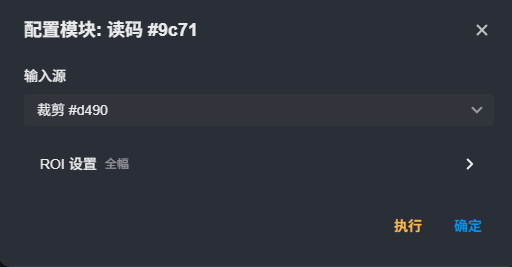
How It Works

After receiving the input image, the code reading module locates and recognizes the code symbol in the image and extracts its encoded content as the result output. The algorithm model used is specified by the "Model ID" parameter, and its value rules are consistent with those of the crop node. In the current version, this module is not yet available in the toolbox, so the related configuration cannot be completed through the regular interface.

Use Cases

Reading code patterns on product packaging and labels.
Automatic collection and traceability of material code information during production.
Inspection tasks that need to convert the code content in the image into text data.

Deep Learning

Deep learning refers to using deep learning models similar to brain neural networks to enable computers to learn and understand complex information and complete difficult recognition tasks. It can be used in scenarios such as image localization and segmentation.

Modules in this category only need model file configuration. Model files are obtained from AIC (AI Creator) based on training with large amounts of sample data.

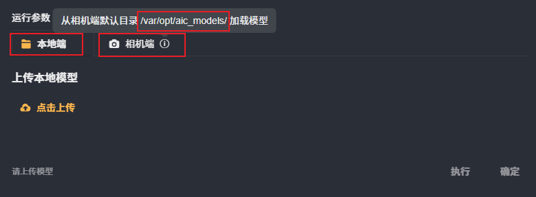
Model Configuration:
- Local
  Download the model trained by AIC to local storage, then upload it.
- Camera
  Since AIC supports deploying trained models directly to integrated cameras, modules in this category scan the model files in the camera's specific directory /var/opt/aic_models, supporting model type parsing and quick selection, eliminating the download and upload steps - convenient and fast. As shown below:

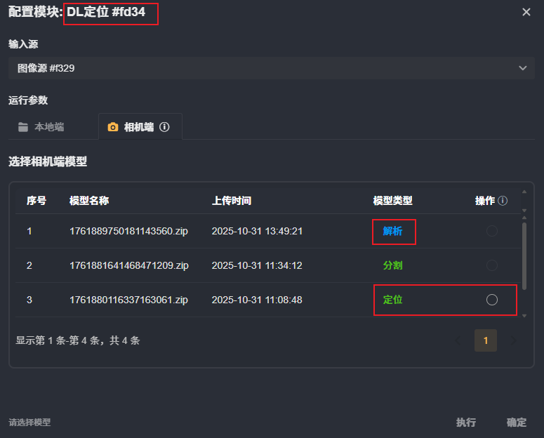
Output Results:
- Model Structure Information
  - Input Shape
  - Output Shape
- Image Results
  - Display intermediate result images after model inference (for example, feature maps, segmentation maps, etc.)
  - Each intermediate result can be viewed and exported separately
As shown below:

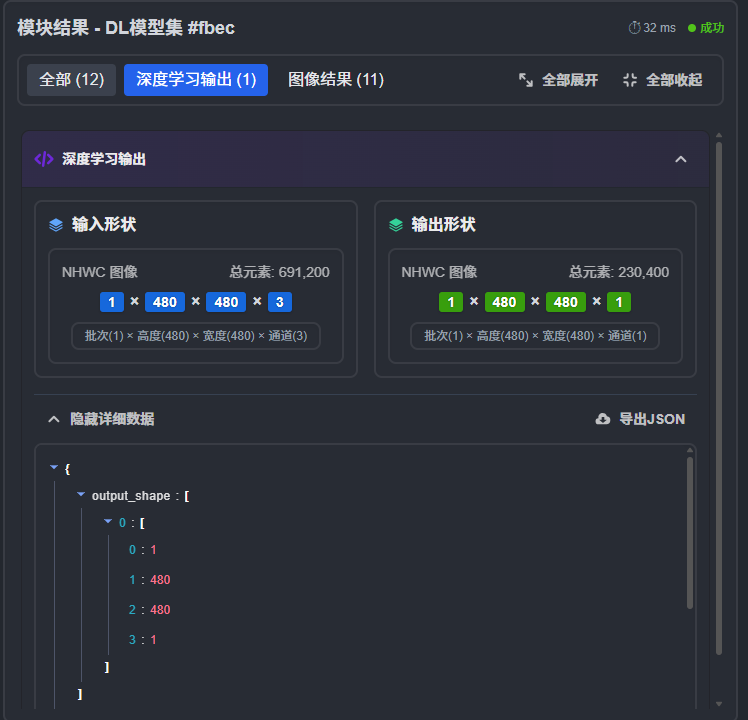
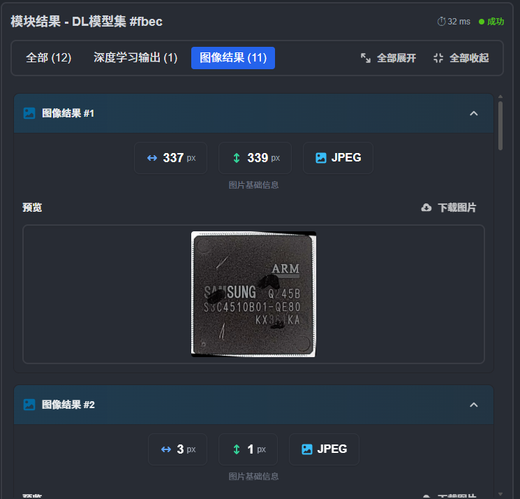
DL Localization

Precisely locates the inspection area, used to determine the object position and mark bounding boxes. The image below shows the result obtained through a localization model.

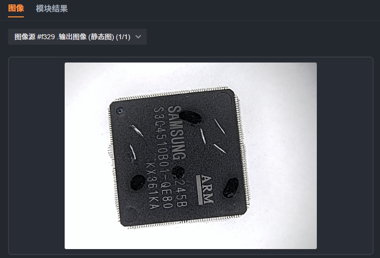
Original Image

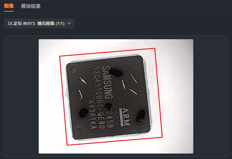
Localization Result Image

As shown in the example steps below, use the localization model to quickly mark the target area with a bounding box. Other deep learning modules operate similarly.

Build the workflow: Image Source -> DL Localization.

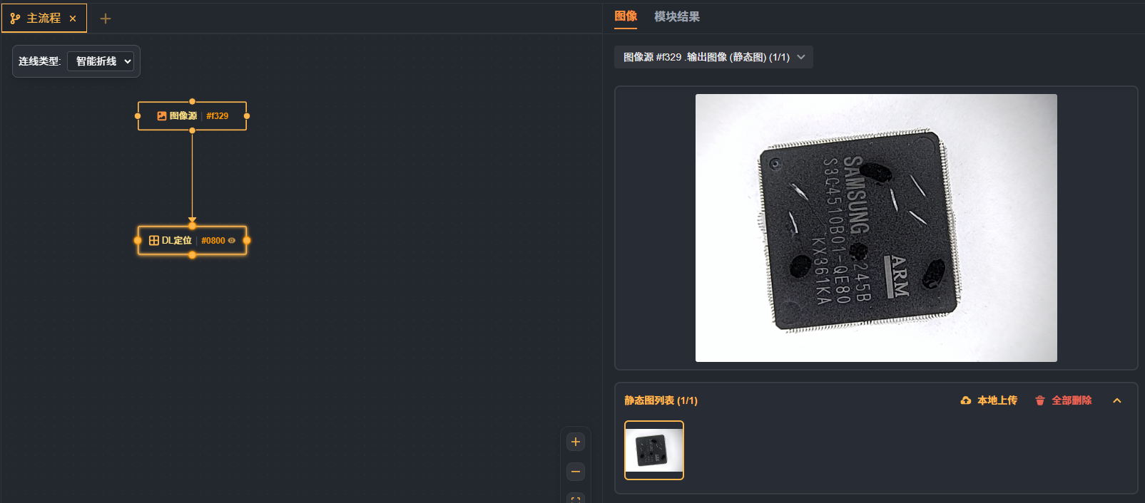
Configure DL Localization: After selecting the corresponding model, detailed information about the model is displayed synchronously, including the Model Name, Target Platform, Quantization Precision, and Version. Click "Execute".

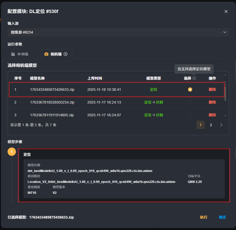
Complete the marking of the target, as shown in the red box area below.

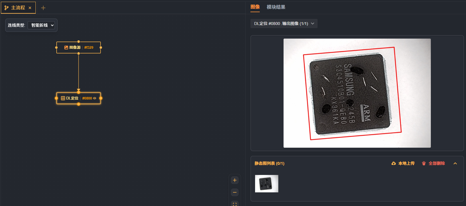
DL Segmentation

Pixel-level processing, commonly used to detect fine defects on the target surface, such as contamination, scratches, and so on. The image below shows the result obtained through a segmentation model.

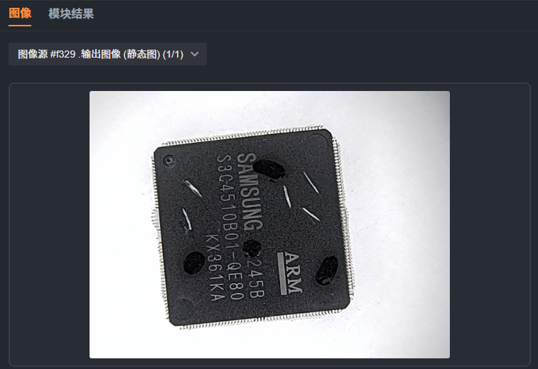
Original Image

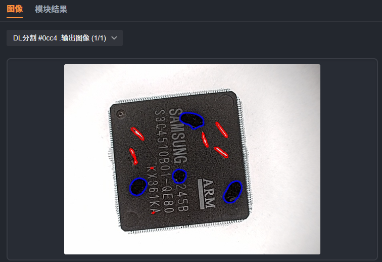
Segmentation Result Image

DL Model Set

When AIC deploys models directly to an integrated camera, it supports packaging the models corresponding to multiple algorithm modules together for unified deployment. For this purpose, the module that supports serial processing of multiple models is the DL Model Set.

Currently, this module only supports selecting a model set that combines the localization and segmentation types. Support for other model types, such as classification, object detection, and OCR, will be added later.

As shown below,

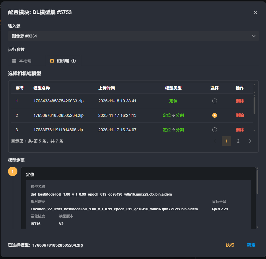
DL Classification

The classification module uses deep learning technology to automatically determine the class of the input image and can quickly recognize the specific class of the target object contained in the image. When the production site needs to sort, grade, or classify defects of products according to visual features, this module can be integrated into the inspection flow to achieve intelligent understanding of image content, replacing manual judgment and improving consistency and efficiency.

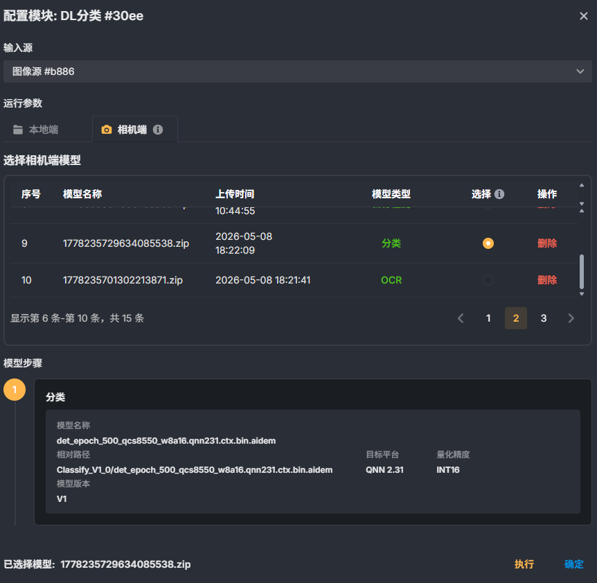
How It Works

The module receives an input image and feeds it into a pre-trained deep learning classification model. The model extracts multi-level features of the image through a convolutional neural network and compares them with the learned feature patterns of each class, and finally outputs the probability value of the image belonging to each class. The module automatically selects the class with the highest probability as the classification result and attaches the corresponding confidence score. When image features are blurred or interference is present, unreliable classifications can be filtered out through the confidence threshold to ensure the reliability of the output result. The whole process requires no manually defined features; you only need to provide representative samples during the training stage.

Use Cases

Product Grading: Distinguish products into different grades such as premium products, first-class products, and defective products according to appearance features.
Defect Classification: Recognize the type of surface defects on products, such as scratches, dents, and contamination, to facilitate subsequent statistical analysis.
Character Recognition Assistance: Classify the image of a single segmented character as a letter, digit, or symbol for combined recognition.
Material Verification: Confirm the model of incoming materials during the assembly process to prevent wrong materials from being mixed in.

Steps

Drag the "Classification" module into the workflow editing area in Smart Vision Studio.
Connect the image input source to the module port.
Specify the deep learning classification model to be used in the module properties (import it in advance through model management).
Run the workflow and view the classification result and confidence output by the module.

Notes

The resolution and channel count of the input image should be consistent with those during model training; otherwise, inference may fail or accuracy may decrease.
The classification model must be imported in advance in "Model Management", and make sure that the model file is compatible with the current software version.
If the confidence threshold is set too high, correct classifications with inconspicuous features may be missed; if it is set too low, incorrect results may be introduced. It is recommended to tune it based on actual samples.
If the classification model requires specific preprocessing (such as a normalization method), confirm that the preceding modules have completed the corresponding processing, or use the preprocessing module built into the software.

Object Detection

The object detection module is based on deep learning technology and can automatically identify and locate the targets of interest in an image. The module receives one or more input images, performs inference through a loaded pre-trained model, and outputs the class, position, and confidence of each target. It is widely used in scenarios such as part recognition, defect localization, and packaging inspection in industrial machine vision, helping users quickly obtain structured target information without manually interpreting images one by one.

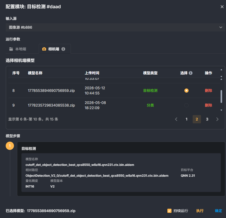
How It Works

The module first reads the input image and feeds it into the configured deep learning object detection model. The model extracts multi-scale features from the image and generates a series of candidate target regions, then determines the class and precise position of each target through classification and bounding box regression networks. After inference is complete, the module filters out results with low reliability according to the set confidence threshold and keeps the target boxes that meet the conditions. Finally, the detection results are output in a standard format, including class labels, confidence scores, and the coordinates of the rectangular bounding box. The whole process is completed automatically and has strong adaptability to complex backgrounds and changes in object shape.

Use Cases

In electronic assembly, detect whether components on a circuit board are present, misaligned, or of the wrong model.
On food packaging lines, recognize the position and content of labels, production dates, or QR codes.
In logistics sorting systems, locate packages of different sizes and shapes to assist robotic arm picking.
In automotive manufacturing workshops, check the integrity and position of small targets such as body weld spots, nuts, and bolts.

Steps

In the scheme editing area, drag the "Object Detection" module from the "Deep Learning" category into the workflow.
Connect the image source (such as the camera acquisition module or the image reading module) to the input port of this module.
Double-click the module to open the property configuration panel, and select the model file that matches the detection task.
Save the configuration and run the workflow; the module performs detection on each input image.
Observe the detection results in the image display area, or connect subsequent modules to filter and otherwise process the target data.

Notes

The model file must match the current detection scenario; if the product under inspection or the process is changed, retrain or replace the model.
The confidence threshold directly affects the number and reliability of the results: raise the threshold appropriately when high accuracy is required, and lower it appropriately when missed detections need to be reduced.
The size and aspect ratio of the input image should be consistent with those during model training; otherwise, detection accuracy may be affected. It is recommended to add an image scaling or cropping module before this module for preprocessing.
NPU inference can significantly improve the processing speed, but make sure that the corresponding graphics driver and inference acceleration library are installed on the industrial PC.
High-resolution images increase the time required for a single inference; on the premise of ensuring the detection effect, you can appropriately reduce the image size to improve the cycle time.

OCR

The OCR module uses deep learning technology to recognize characters in an image and convert the text regions in the image into editable, searchable text information. This module is suitable for industrial scenarios such as product label reading, packaging inkjet code recognition, and character extraction from engraved metal parts. It can replace manual entry and significantly improve the information collection efficiency and accuracy of automated systems.

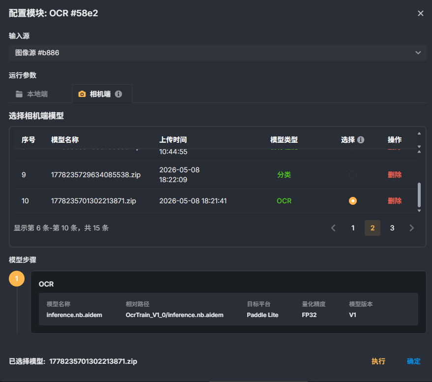
How It Works

After preprocessing the input image, the OCR module detects the text regions in the image through a pre-trained deep neural network model and performs end-to-end recognition of the character sequence in each region, finally outputting structured text content. The processing flow can be summarized as follows: receive the image to be detected, automatically locate text lines or character blocks, parse the semantics of the characters line by line, fuse context information to improve recognition accuracy, and finally output the recognition result text as well as the confidence of each character. Users only need to select a suitable model to adapt to text recognition tasks with different fonts, sizes, and backgrounds.

Use Cases

Recognize and record the production date, batch number, and expiration date on product packaging.
Extract the model numbers and serial numbers laser-engraved on the surface of electronic components.
Automatically read and verify characters on metal nameplates or labels.
Batch entry of printed or standard handwritten information on receipts and forms.

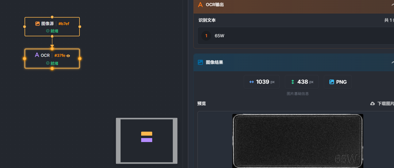
Steps

In the Smart Vision Studio workflow, add the OCR module from the "Deep Learning" category.
Connect the upstream image output port to the input port of the OCR module, and make sure that the incoming data is image data containing the text to be recognized.
Select a preset OCR model in the parameter settings area; you can choose the best-matching model according to the character type (digits, letters, Chinese, and so on) and the background complexity.
Run the workflow, view the recognized text content and confidence in the result area, and adjust the parameters or the ROI according to the result.
Connect the output of the OCR module to subsequent data processing or logical judgment modules to complete the automation integration.

Notes

The clarity of the input image directly affects the recognition accuracy. It is recommended to add image enhancement or preprocessing steps before the OCR module, such as contrast enhancement and denoising.
Model selection should match the actual character set; for example, prefer a model dedicated to digits when recognizing pure numeric sequences to obtain higher accuracy.
Text regions that are too small or characters that are too densely spaced may cause missed detections; this can be solved by adjusting the image acquisition resolution or by combining a localization module to enlarge the target region.
The inference speed is affected by the image resolution and the model complexity. On high-speed production lines, evaluate whether the processing time meets the cycle time requirements.
If the confidence of the recognition results is generally low, check the stability of the light source and the printing quality of the characters, or try a more general pre-trained model.

Text Detection

The text detection module is based on deep learning technology and allows you to enter a natural language description (such as "silver screw" or "barcode") to automatically find and box out all targets in the image that match the description. This module combines language understanding with visual detection and gets rid of the dependence of traditional algorithms on fixed features; it is especially suitable for detection tasks with multiple varieties, small batches, or non-fixed defect shapes. Choose this module when you need to locate targets in an image according to flexible semantic rules.

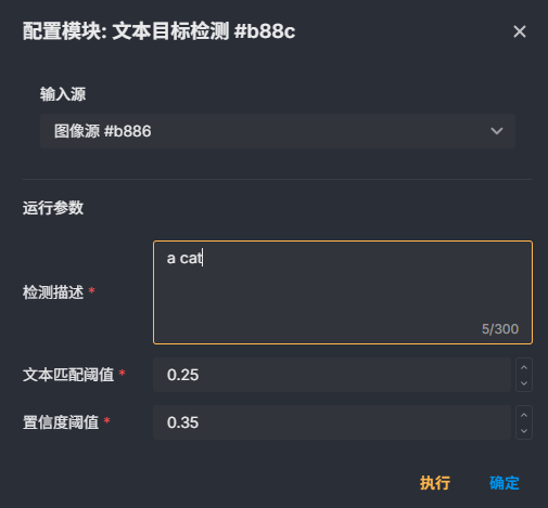
How It Works

The module receives the image to be detected and a text instruction describing the target features, and then feeds both into a pre-trained deep learning model. The model parses the image content and the text meaning at the same time and searches the image feature space for regions that are highly consistent with the text description. The module then filters out the target boxes that meet the conditions according to the preset confidence threshold and outputs their position, size, and corresponding confidence. The whole process is completed entirely in the inference stage, with no need to retrain for each type of target, which greatly lowers the deployment barrier. This method is especially suitable for scenarios that need to quickly adapt to new objects or defects, such as locating different workpieces on a flexible production line and capturing unknown defects.

Use Cases

Workpiece Sorting: Enter "silver screw" to quickly locate all similar parts in the image.
Character and Pattern Localization: Describe "barcode" or "logo" to directly box out the printed area and provide input for subsequent OCR or comparison.

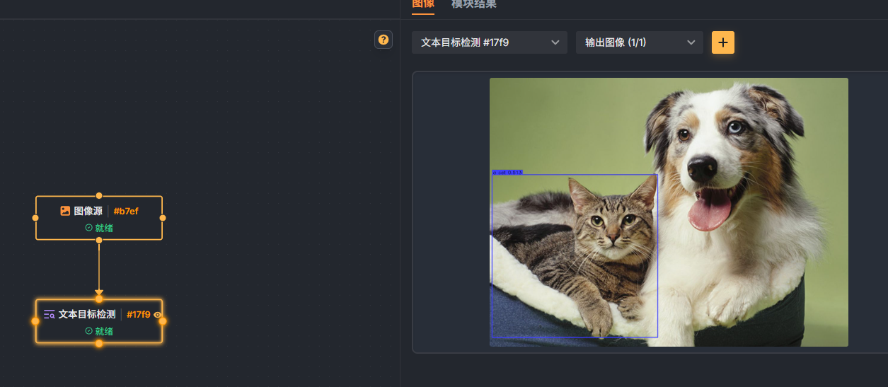
Parameters

Parameter	Description	Default Value
Text Prompt	A natural language description string that tells the module what target to look for in the image. The description should be as specific as possible; avoid vague words.	None (manual input required)
Box Threshold	The lower confidence limit for filtering detection boxes. Detection results below this value are discarded. Raising the threshold reduces false detections, and lowering it improves the recall of weak targets.	0.3 (a typical setting for the task)
Text Threshold	The minimum requirement for the similarity of the text-image match. This threshold affects how strictly the model judges the association between the text description and the visual features. The higher the threshold, the more conservative the results, keeping only matches with high certainty.	0.25 (a typical setting for the task)

Steps

In the flow editing interface, drag the "Text Detection" module from the "Deep Learning" category into the workflow.
Connect the upstream image input to the "Image Source" entry of this module.
In the module parameter panel, click the model selection drop-down list and choose the detection model suitable for the current task.
Type the target description in the "Text Prompt" input box, for example "a cat" or "a apple".
Adjust the "Box Threshold" and "Text Threshold" as needed. For the first run, you can use the default values and fine-tune them later according to the detection effect.
Click the run button; the system performs inference and displays the detected target boxes and confidence information in the output area.
If you need to continue processing the detection results, connect the module output to subsequent localization, counting, or measurement steps.

Notes

The accuracy of the text prompt directly affects the detection effect. Use expressions that are common in model training, avoid rare words or overly abstract sentences, and note that only English is supported.
The box threshold and the text threshold together determine the number of targets in the final output. It is recommended to observe the confidence distribution of typical images first and then set a reasonable cutoff value, instead of blindly using the default values.
Different models have different sensitivity to text length; an overly long text description may degrade the matching effect, so use concise phrases.
The resolution and clarity of the input image affect the performance of small target detection. For targets smaller than 32×32 pixels, try enlarging the local region through preprocessing.
Running the module requires a certain amount of computing resources. With large high-resolution images or in multi-target scenarios, the inference time may increase; choose a suitable model according to the cycle time requirements.

Result Processing and Visualization

Result Rendering

Result rendering means that, according to the start node and end node specified in the flow, the results produced by each intermediate processing module (such as detection boxes, contours, and key points) are rendered uniformly onto the target image for result display and visualization output.

This function is commonly used to debug a flow, verify results, and display the final image output.

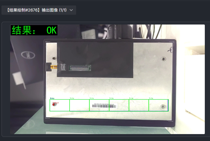
Overview

Collect the processing results within the specified node range in flow order
Overlay and render the detection results of each module onto the image
Support unified visualization of multiple result types (such as boxes, points, contours, and so on)
Output an image with annotation information

Parameters

Start Rendering Node Specifies the starting node for rendering; result data collection starts from this node.
End Rendering Node Specifies the ending node for rendering; result data collection stops at this node.

Merge Block Results

Merge block results is used to restore the target detection, image segmentation, or classification results obtained by dividing a large image into grid blocks and analyzing them separately, back into the coordinate system of the whole image. It can handle overlapping regions between blocks, remove duplicate results for the same target, and merge targets that cross block boundaries into complete targets, generating a whole-image result that can be used directly for viewing, statistics, and subsequent analysis.

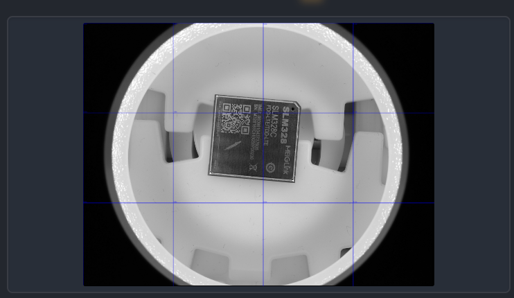
How It Works

The module reads the analysis result of each block and its position information in the whole image. First, the coordinates in each block result are converted into whole-image coordinates based on the block origin. Then the overlapping regions between adjacent blocks are checked, and results that represent the same target are matched. Matching comprehensively considers the degree of positional overlap, class consistency, and confidence, and decides, according to the strategy set by the user, which one to keep or whether to fuse them into a new result. For a single target cut apart by block boundaries, if it appears separately in different blocks, the module merges them into one complete target. Finally, it outputs the whole-image result under unified coordinates and a unified class system.

Logical Judgment

Result Filtering

Result filtering means that based on the detection results output by the parent node (such as Blob, contours, and so on), targets are filtered according to the set conditions, and only the results that meet the conditions are kept, so as to improve the detection accuracy or remove invalid targets.

This module is usually used to remove noise, small targets, or regions that do not meet the feature requirements, and is an important step in result post-processing.

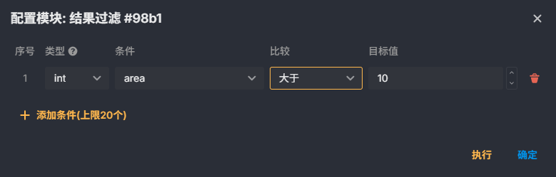
Overview

Filter based on the result data of the parent node
Support multiple attribute conditions (such as area, length, grayscale, and so on)
Support multiple data types and comparison methods
Output the set of targets that meet the conditions

Parameters

Type Specifies the data type involved in the comparison:
- int: Integer type (such as the number of pixels)
- float: Floating-point type (such as the grayscale mean, ratio, and so on)
- string: String type (such as the classification label, and so on)
Condition Specifies the attribute field to filter by:
- area: Area (number of pixels)
- length: Length (such as the contour perimeter or the boundary length)
- grayscale: Grayscale value (such as the mean or a specified statistic)
Comparison Method
- Equal to (=)
- Less than (<)
- Less than or equal to (≤)
- Greater than (>)
- Greater than or equal to (≥)
- Range: Within the specified range (inclusive or exclusive of the boundaries, depending on the implementation)
Target Value
- When the comparison method is a single-value comparison: enter one target value
- When the comparison method is a range: enter the minimum value and the maximum value

Condition Judgment

Condition judgment means that based on the output result of the specified parent node, a set of filtering conditions is configured to perform a logical judgment on the result, and the overall judgment result (OK / NG) is output.

This module does not directly filter or modify the result data; instead, it is used for flow control and the final quality judgment.

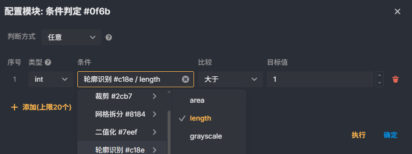
Overview

Perform a condition judgment based on the result data of any parent node
Support combined judgments with multiple conditions
Support different logical relationships (ANY / ALL)
Output the overall judgment result (OK / NG)

Parameters

Judgment Method
- All Satisfied (ALL) When all conditions are satisfied, the result is OK; otherwise, it is NG
- Any Satisfied (ANY) When any one condition is satisfied, the result is OK; otherwise, it is NG
Type Specifies the data type involved in the comparison:
- int: Integer type (such as area, quantity)
- float: Floating-point type (such as the grayscale mean, ratio, and so on)
- string: String type (such as a label)
Condition Specifies the attribute field involved in the judgment:
- area: Area
- length: Length (such as the contour perimeter)
- grayscale: Grayscale value
Comparison Method
- Equal to (=)
- Less than (<)
- Less than or equal to (≤)
- Greater than (>)
- Greater than or equal to (≥)
- Range
Target Value
- Single condition: Enter one target value
- Range: Enter the minimum value and the maximum value

Output Results

OK: The configured judgment logic is satisfied
NG: The configured judgment logic is not satisfied

Communication

Modules under the Communication category primarily implement camera-to-external-device communication functionality.

IO Output

This module is mainly used for level control of output pins. It supports level control for 4 IO ports. The mapping is as follows:

	I/O Signal Source	Description	Cable Color Reference
IO0	Line4	Opto-isolated Output 4+	Green
IO1	Line5	Opto-isolated Output 5+	Yellow
IO2	Line3	Opto-isolated Output 3+	Black
IO3	Line6	Opto-isolated Output 6+	Gray

Parameter Configuration
- Output Condition: You can subscribe to the output conditions for each IO output signal. Currently, only subscribing to the output results of preceding modules is supported. When the preceding module executes successfully, this output condition is triggered.
- Duration (ms): When the duration is greater than 0, it means that after the level is pulled high, the level is automatically pulled low after the corresponding duration. When it is 0, no level-low action is performed.
- Output Type: Output on OK, output on NG

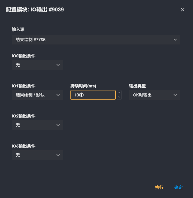
Output Results
The result panel displays the output status of each channel. 0 indicates the current level is low, as shown below:

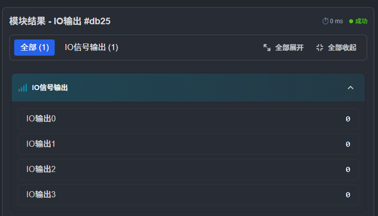
Extension

Custom Operator

Custom operators are used to extend system capabilities. They allow users to implement custom algorithm logic according to the provided interface specification (header file) and integrate it into the flow as a dynamic library (.so) for execution.

This module is suitable for special requirements that standard operators cannot cover, such as custom detection logic, complex business rules, or third-party algorithm integration.

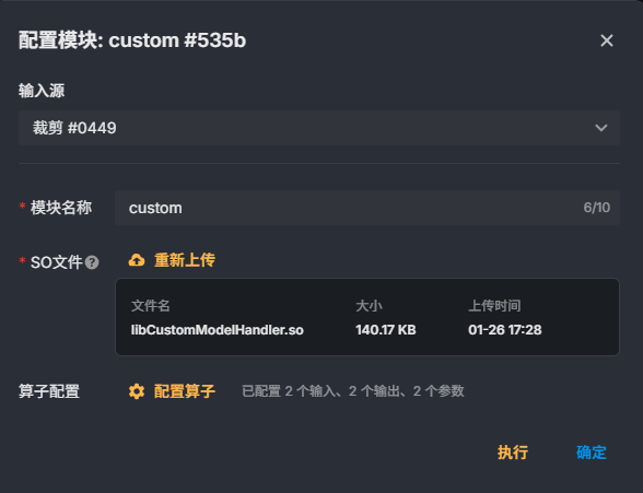
Overview

Support loading user-defined dynamic libraries (.so)
Call custom algorithm logic through the agreed interface
Support standardized input and output data structures
Can participate in full flow orchestration and connect seamlessly with other modules

Parameters

Module Name The module name defined by the user, used to identify this operator in the flow.
so File The dynamic library file (.so) implemented by the user, which contains the specific algorithm logic.
Operator Configuration Defines the input, output, and runtime parameters of the operator, uniformly described in a Key-Value structure.

Operator Configuration Description

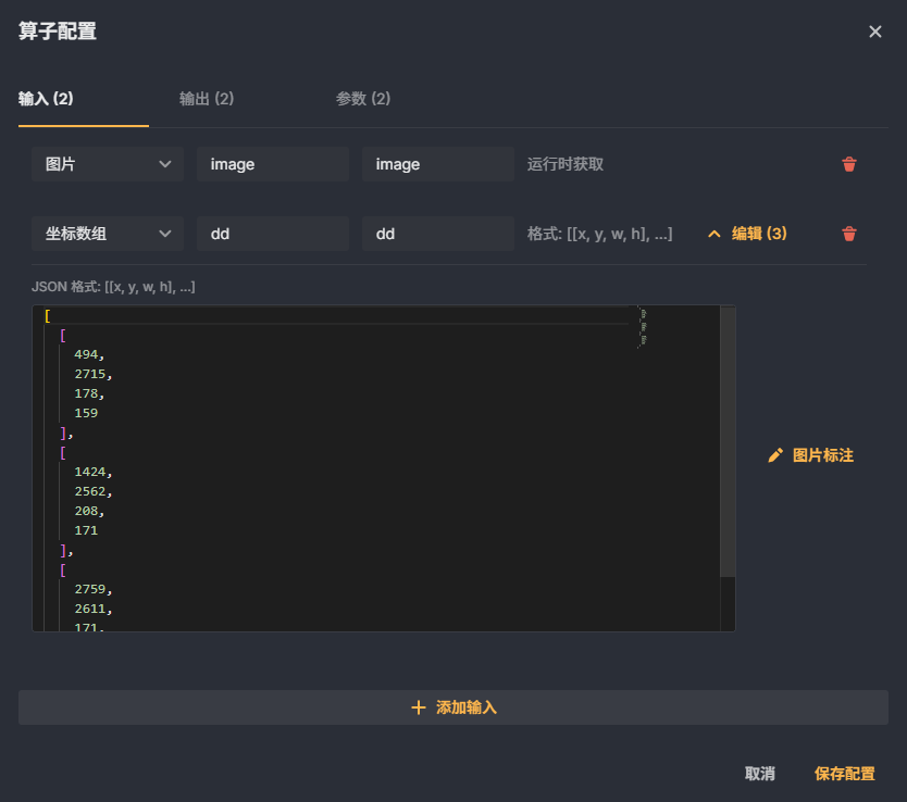
The operator configuration is divided into three categories: Input, Output, and Params. Each item consists of the following structure:

Type: Data type
Name: Display name
key: Field identifier
value: Actual data or default value

Input

Used to receive data from upstream nodes. Supported types:

Image
Number (int / float)
String
Boolean (bool)
Coordinate array (such as point sets, contours, and so on)

Output

Used to pass results to downstream nodes. Supported types:

Image
Number (int / float)
String
Boolean (bool)
Coordinate array

Params

Used to configure the runtime parameters of the operator's internal logic. Supported types:

Number (int / float)
String
Boolean (bool)
JSON (used for complex structure configuration)

Notes

A custom operator must strictly follow the interface specification (header file) provided by the platform; otherwise, it may fail to load or run abnormally. The header file reference is as follows:

#ifndef __CUSTOMMODELHANDLER_H__
#define __CUSTOMMODELHANDLER_H__

#include <opencv2/opencv.hpp>
#include <jsoncpp/json/json.h>

namespace CustomModel {

/**
 * @brief Initialization parameter struct
 */
struct InitInfo
{
    /// Folder path used to store the data operated on by the custom module
    std::string customDirPath;

    /// JSON configuration object configured on the web page
    Json::Value configureJson;
};

/**
 * @brief Image type enum
 */
enum ImageType
{
    Empty = 0,   ///< Empty image
    Origin,      ///< Original image
    Mask,        ///< Mask image
    Result       ///< Result image
};

/**
 * @brief Input parameter struct
 */
struct InputInfo
{
    ImageType imageType {Empty};  ///< Image type

    cv::Mat image;                ///< Image data

    /**
     * @brief May be empty; the JSON object of the input part of the web page configuration file
     */
    Json::Value params;
};

/**
 * @brief Output parameter struct
 */
struct OutputInfo
{
    ImageType imageType {Empty};  ///< Image type

    cv::Mat image;                ///< Image data

    /**
     * @brief May be empty; the JSON object of the output part of the web page configuration file
     */
    Json::Value params;
};

/**
 * @brief Processing parameter struct
 */
struct HandleInfo
{
    std::vector<InputInfo> inputInfoList;   ///< Input information list
    std::vector<OutputInfo> outputInfoList; ///< Output information list
};

/**
 * @brief Model handler class
 */
class Handler
{
public:
    virtual ~Handler() = default;

    /**
     * @brief Initialize the model and related parameters through the configuration
     * @param initInfo Initialization parameter struct
     * @return Initialization result (0 means success, non-0 means failure)
     */
    virtual int init(const InitInfo& initInfo) = 0;

    /**
     * @brief Use the model to process the input image to obtain the output result
     * @param handleInfo Processing parameter struct
     * @return Image processing result (0 means success, non-0 means failure)
     */
    virtual int handleImage(HandleInfo& handleInfo) = 0;

    /**
     * @brief Release the resources occupied while using the model
     * @return Resource release result (0 means success, non-0 means failure)
     */
    virtual int release() = 0;
};

} // namespace CustomModel

extern "C" {
    /**
     * @brief Create a handler instance
     * @return Handler instance pointer
     */
    CustomModel::Handler* create_instance();
    
    /**
     * @brief Delete a handler instance
     * @param handler The handler instance pointer to delete
     */
    void delete_instance(CustomModel::Handler* handler);
}

#endif // __CUSTOMMODELHANDLER_H__

The input and output fields must remain consistent with the data types of the upstream and downstream nodes in the flow.

Debugging and Running

This chapter describes how to run a flow, how to troubleshoot problems node by node, and how to view results and duration.

Running Modes Overview

Method	Entry	Running Scope	Applicable Scenarios
Full-flow execution	Execute in the top action bar	All nodes in the current flow	Verify a complete solution, formal running
Single-node execution	Execute at the bottom of the node configuration dialog	The current node only	Quickly check the effect after adjusting a parameter, locate the problem node

Note: Both methods are "save then run" - before clicking run, the current workflow is saved to the device first.

Pre-run Checks

Complete connections: Except for acquisition nodes, every node should have an upstream input; when no input source is selected, Execute and OK in the dialog are unavailable.
Valid input source: The Input Source drop-down in the node dialog should display a specific node, not "Please select an input node".
Valid parameters: For example, Circle Finding requires that "Minimum Sector Ring Radius" is not greater than "Maximum Sector Ring Radius".
Camera available: If the camera is already occupied by another application, a prompt appears when running; you can choose to close the occupying program and try again.
Converged flow: A multi-branch flow must finally merge into one output node; if an unconverged branch exists, the flow cannot be executed.

Full-flow Execution

Click Execute in the top action bar (the tooltip text is "Execute the current workflow").
During running, the page displays a full-screen mask Workflow executing...; do not click repeatedly at this time.
After running ends:
- The bottom summary bar shows the overall status of this run;
- The result panel on the right refreshes to the images and module results of this run.
If the flow contains static image nodes, the run uses the image currently selected in each static image node.

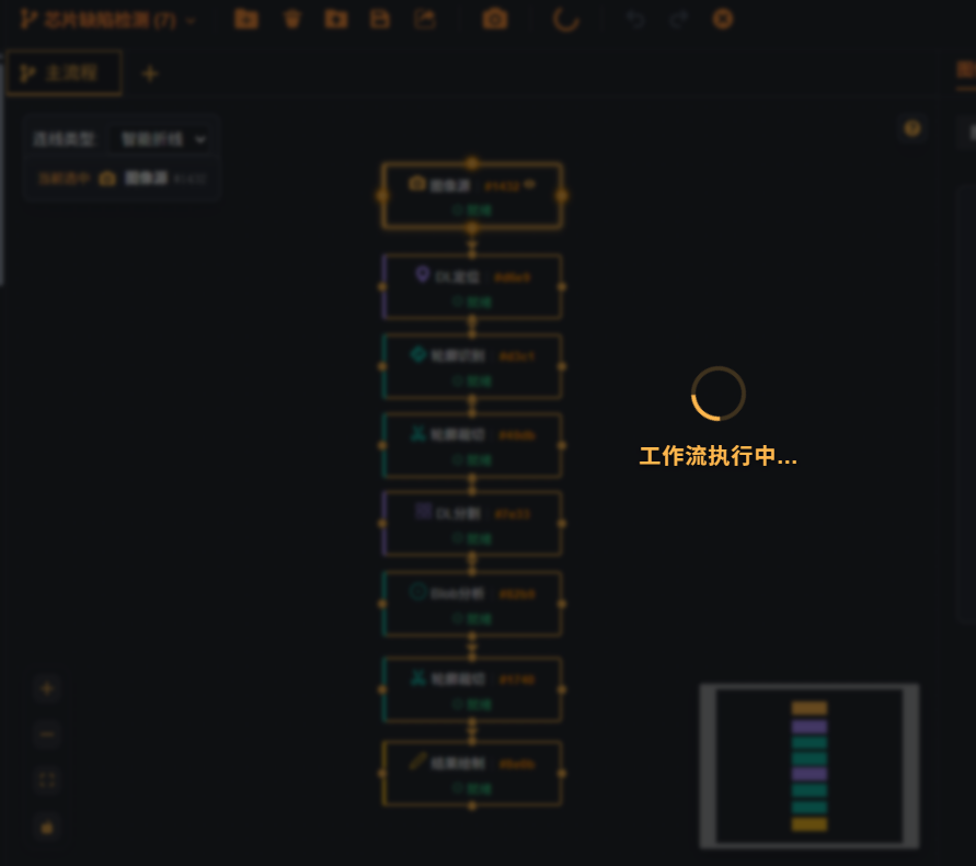
Single-Node Execution (Single-Step Debugging)

For the scenario of "only changing one node and only looking at that node":

Double-click the target node on the canvas to open the configuration dialog.
After modifying the parameters, click Execute at the bottom of the dialog (if you only want to save the parameters, click OK).
The system saves the workflow and then runs only this node; when the run ends, the result panel on the right refreshes to the output of this node.

Differences from full-flow execution:

Item	Full-flow Execution	Single-node Execution
Running scope	All nodes	The current node only
Upstream data	Regenerated by this run	Reuses the existing run results of upstream nodes
Typical use	Complete solution verification	Single-point parameter tuning, locating the problem node

Key points for use:

Single-node execution does not re-run upstream nodes, so the upstream node must have run at least once and produced output; otherwise this node may fail due to a missing input image or data.
The node must be enabled; a disabled node cannot be executed on its own.
Single-node execution also refreshes the duration and status of this node, which can be used to judge the impact of a parameter change on performance.

Result Verification

After running, verify in the order of "from the whole to the parts":

1. Look at the Overall Result

The bottom summary bar shows: total flow duration, selected module duration, module count, and result (success/failure). When the overall result is abnormal, first locate the specific node and then look at the details.

2. Verify Node by Node

Switch the panel on the right to the Module Results tab and select a node in the drop-down. The list header shows the following for that node:

Duration (ms);
Status: success (green) / failure (red);
On failure, an error message is given (hover over the warning icon to view the specific cause).

Different modules have different result contents (circle center coordinates and radius, measured values, classification results, OCR text, and so on)

3. Look at the Image

Switch to the Image tab to view the output image, and judge whether the localization boxes, measurement annotations, and rendering results meet the expectations; use the pixel probe to verify the local grayscale values when necessary.

4. Verify by Image (Static Image Flow)

When static images are used as input, each image has its own run record and status, and the corresponding status is marked in the static image list; the "total flow duration" in the bottom summary bar is the sum of the durations of the images. For troubleshooting, it is recommended to first find the images with an abnormal status, and then go back to the corresponding node to verify the result of that image.

5. Save the Results

The result panel provides a download entry, which can save the node output (image or result file) to the local device for comparison with a host system or historical data.

Verification Tips

First verify the flow with an image whose result is already known, and run it in batches only after confirming that it is correct.
For flows that involve localization/measurement, it is recommended to use the Result Rendering module to overlay the results on the image and confirm them quickly by eye.
For numeric results, focus on verifying the order of magnitude and the unit (pixels / physical units after calibration).

Duration Analysis

Available Duration Data

Location	Content
Bottom summary bar	total flow duration (the sum of the durations of the images), selected module duration (shown after a canvas node is selected), module count
Module Results tab	Duration (ms) and status of the selected node
Node run records (saved in the background, not shown in the UI)	Total duration of each node and the durations of the three stages of preprocessing, algorithm invocation, and postprocessing

Analysis Steps

Look at the total: compare whether the "total flow duration" is stable across multiple runs; a large fluctuation indicates random factors (camera stream grabbing, first-time model loading, system load).
Find the hotspot: select the nodes on the canvas one by one, and find the node with the highest proportion from the "selected module duration" or from the duration in the module results.
Break down the stages: the background run records split the node duration into three stages: preprocessing, algorithm invocation, and postprocessing; if preprocessing takes a high proportion, it is usually the cost of image reading/conversion, and if algorithm invocation takes a high proportion, it is related to the algorithm parameters, the ROI size, and the image size.
Align with the requirements: confirm whether the duration of a single run meets the production line takt; for continuous running, the overlap between stream grabbing and processing must also be considered.

Common Optimization Directions

Reduce the processing range: set the ROI properly to avoid a full-image search.
Reduce the amount of computation: reduce parameters such as the number of calipers, the number of templates, and the maximum number of results; for matching modules, limit the angle and scale range.
Enable acceleration options: finding modules can enable initial localization (coarse first, then fine).
Downscale the image: use image scaling to reduce the resolution while the accuracy requirement is met.
Model selection: for deep learning modules, prefer a model that matches the accuracy requirement.

Notes

The first run is slower: one-time costs such as camera initialization and model loading make the first run noticeably slower than later runs; it is recommended to use the duration of the second and later runs as the reference.
Running multiple images: for batch static image runs, the "total flow duration" is the sum of the durations of multiple images; when evaluating the takt of a single run, convert it according to the number of images.
Look at duration and results together: after parameter tuning, confirm both that the duration decreases and that the results are still correct.

Q: After clicking "Execute", the spinner keeps turning?

A: Check whether the camera is occupied by another program and whether an image has been selected for the static image; you can stop and then run again.

Q: The node fails when executed on its own, but full-flow execution works?

A: Single-node execution reuses existing upstream results; run the complete flow once first, and then debug this node on its own.

Q: Why do the results not change after the parameters are changed?

A: Confirm that you clicked Execute or OK in the dialog and that the save has completed; if you clicked Execute, the system saves first and then runs this node.

Appendix

Glossary

Term	Description
Workflow	A complete vision solution, including flows, nodes, and connections
Flow	A branch in a workflow, presented as a canvas tab
Node / module	A functional unit on the canvas (such as Circle Finding or Measurement)
ROI	Region of interest, used to limit the detection range
Caliper	A form of ROI that arranges detection units along a specified direction
Edge polarity	The light-dark transition direction of the detected edge (any/from black to white/from white to black)
Initial localization	An acceleration mechanism that performs coarse localization at a low resolution first and then fine localization on the original image
Calibration	The process of establishing the conversion relationship between pixel coordinates and physical coordinates
Pixel scale	The physical size corresponding to each pixel
Model set	A set that organizes multiple deep learning models to be used as one node
IO Output	Output high and low level signals through the device IO interface

FAQ

What operations auto-save? Which operations require manual save?

Debounced auto-save (triggered 2 seconds after editing): all canvas editing operations such as dragging nodes, deleting nodes, creating/deleting connections, moving nodes, clearing the canvas, and undo/redo
Immediate save (triggered before the operation): double-clicking a node to open the configuration dialog, executing the current workflow, and exporting an app; these operations save first and then continue, ensuring they act on the latest state
Silent save: automatically save the current workflow when switching workflows (no prompt shown)
Manual save: click the "Save to Camera" button in the top toolbar

Important:

Debounced auto-save has a 2-second delay. If you close the page within 2 seconds of editing,

your edits may be lost. To ensure they are persisted immediately, click the "Save to Camera" button.

How to choose between Camera and Static Image?

Drag the Image Source node to the canvas (defaults to Camera node)
Double-click the Image Source node to open the configuration dialog
Select "Camera" or "Static Image" from the top dropdown
The corresponding configuration form is displayed below

How to delete a node?

Right-click a node (the node is highlighted with a dashed border)
You can continue right-clicking other nodes for multi-selection
A delete operation panel appears automatically
Click the delete button to delete all selected nodes
Click a blank area of the canvas to deselect

Do nodes already have default parameters after being dragged?

Yes. Default parameters are written automatically when a node is dragged onto the canvas (for example, the camera defaults to C0), and they take effect without waiting for configuration.

Camera node: NodeName #ShortID .Output Image(C0 Camera) (1/1)
Static Image node: NodeName #ShortID .Output Image(Static Image) (1/1)
Other processing nodes: NodeName #ShortID .Output Image (1/1)

The ShortID is the last 4 characters of the node's full ID, used to distinguish nodes of the same type.

How to upload and manage static images?

: Double-click the Image Source node and select the "Static Image" type
: The "Static Image List" panel is displayed on the right
: Click the "Upload Local File" button to select images (multi-select supported)
: Click a thumbnail to switch the display
: Hover over an image and click the trash icon to delete a single image
: Click the "Delete All" button to delete all images

How to avoid overwriting an existing app when exporting?

When exporting to SVE Camera, the system automatically checks whether an app with the same app ID and version exists
If one exists, a confirmation dialog appears: "The app already exists. Overwrite?"
Select "Cancel" to abort the export, modify the version number, and export again
Exporting to Local does not check for duplicates and downloads the zip file directly

AidLux System

Quick Start

System Flashing

System Usage

System Configuration

Ubuntu System

Quick Start

System Flashing

System Usage

System Configuration

Hardware Description

AI Development

AI App Development (AidLite)

AI Model Conversion

Generative AI App Development

AidVoice SDK

Tutorials

AI Tutorials

Generative AI Tutorials

Voice AI Tutorials

Basic Development

48 PIN GPIO Application

Audio Development

Cross-System Communication

Tutorials

Video Codec Development

Vision Development

Robot Development

Hardware Peripheral Connection

Tool Installation

Resource Summary Download

FAQ

System FAQ

AidLux System

Quick Start

System Flashing

System Usage

System Configuration

Ubuntu System

Quick Start

System Flashing

System Usage

System Configuration

Hardware Description

AI Development

AI App Development

Generative AI App Development

AidGen SDK

AidGenSE

AI Voice Development

AI Model Conversion

Tutorials

AI Tutorials

Generative AI Tutorials

Model Farm Tutorials

Voice AI Tutorials

Basic Development

40 PIN GPIO Application

Audio Development

Cross-System Communication

Tutorials

Video Codec Development

Vision Development

Robot Development

Common Peripherals

Tool Installation

Resource Summary Download

FAQ

System FAQ

Ubuntu System

Quick Start

System Flashing

System Usage

System Configuration

Board Hardware & Interfaces

AI Development

AI App Development

Generative AI App Development

AidGen SDK

AidGenSE